A D-shaped Cylinder#
This demo simulates a D-shaped cylinder, representing an idealized ventricle, coupled to a circulatory model (Bestel model). The active contraction is driven by an activation function derived from the Bestel model.
Problem Formulation#
Geometry: A D-shaped cylinder is used as a simplified representation of a ventricle. It has:
An inner radius \(r_{inner}\) and outer radius \(r_{outer}\).
A flat septum-like wall.
A curved free-wall.
A height \(H\).
Physics: We solve the balance of linear momentum for a hyperelastic material:
Material Model:
Passive: Transversely isotropic Holzapfel-Ogden model.
Active: Active stress model driven by an activation variable \(T_a\).
Compressibility: Compressible formulation (penalty method).
Circulation Coupling: The mechanical model is coupled to a circulatory model (Bestel model) which provides:
Cavity Pressure (\(P_{cav}\)): Applied as a Neumann boundary condition on the inner surface.
Activation (\(T_a\)): Applied as the active tension in the mechanics model.
The Bestel model defines the evolution of pressure and activation over time, representing the cardiac cycle.
Boundary Conditions:
Robin BC (Springs): Applied to the outer surface, top, and bottom to mimic tissue support.
Dirichlet BC: The top and bottom faces are constrained in the z-direction (\(u_z = 0\)) to prevent rigid body motion and mimic the attachment to the valve plane and apex.
Neumann BC: Cavity pressure applied to the inner surfaces (curved and flat).
from dolfinx import log
import ufl
import matplotlib.pyplot as plt
import numpy as np
from scipy.integrate import solve_ivp
import adios4dolfinx
import pulse
import cardiac_geometries
import cardiac_geometries.geometry
import shutil
Setup and Logging#
We set up logging to monitor the simulation progress.
circulation.log.setup_logging(logging.INFO)
comm = MPI.COMM_WORLD
1. Geometry Generation#
We generate a D-shaped cylinder mesh using cardiac_geometries.
This function creates a mesh with specific tags for different surfaces:
INSIDE_CURVED: Inner curved surface (Endocardium Free Wall)
INSIDE_FLAT: Inner flat surface (Endocardium Septum)
OUTSIDE_CURVED: Outer curved surface (Epicardium Free Wall)
OUTSIDE_FLAT: Outer flat surface (Epicardium Septum)
TOP: Top basal plane
BOTTOM: Bottom apical plane
It also generates fiber fields (\(\mathbf{f}_0, \mathbf{s}_0, \mathbf{n}_0\)).
r_inner = 0.02
r_outer = 0.03
height = 0.05
inner_flat_face_distance = 0.015
outer_flat_face_distance = 0.025
# Clean up previous geometry if it exists to ensure a fresh generation
shutil.rmtree(geodir, ignore_errors=True)
if not geodir.exists():
    comm.barrier()
    cardiac_geometries.mesh.cylinder_D_shaped(
        outdir=geodir,
        create_fibers=True,
        # We use Discontinuous Galerkin (DG) elements for fibers to allow for discontinuities at boundaries
        fiber_space="DG_1",
        r_inner=r_inner,
        r_outer=r_outer,
        height=height,
        inner_flat_face_distance=inner_flat_face_distance,
        outer_flat_face_distance=outer_flat_face_distance,
        char_length=0.01,
        comm=comm,
        fiber_angle_epi=-60,
        fiber_angle_endo=60,
    )
D-shaped cylindrical shell mesh generated and saved to cylinder_d_shaped/cylinder_D_shaped.msh
2025-12-15 07:17:24 [debug    ] Convert file cylinder_d_shaped/cylinder_D_shaped.msh to dolfin
Info    : Reading 'cylinder_d_shaped/cylinder_D_shaped.msh'...
Info    : 27 entities
Info    : 282 nodes
Info    : 1348 elements
Info    : Done reading 'cylinder_d_shaped/cylinder_D_shaped.msh'
[12/15/25 07:17:24] INFO INFO:cardiac_geometries.geometry:Reading geometry from cylinder_d_shaped geometry.py:323
# Load the geometry and convert to `pulse.HeartGeometry`
geo = cardiac_geometries.geometry.Geometry.from_folder(
    comm=comm,
    folder=geodir,
)
INFO INFO:cardiac_geometries.geometry:Reading geometry from cylinder_d_shaped geometry.py:323
geometry = pulse.HeartGeometry.from_cardiac_geometries(geo, metadata={"quadrature_degree": 6})
try:
    import pyvista
except ImportError:
    print("Pyvista is not installed")
else:
    # Create plotter and pyvista grid
    p = pyvista.Plotter()

    vtk_mesh = dolfinx.plot.vtk_mesh(geometry.mesh)
    grid = pyvista.UnstructuredGrid(*vtk_mesh)

    # Attach vector values to grid and warp grid by vector
    actor_0 = p.add_mesh(grid, show_edges=True)

    p.show_axes()
    if not pyvista.OFF_SCREEN:
        p.show()
    else:
        figure_as_array = p.screenshot(outdir / "d_cylinder_mesh.png")
2025-12-15 07:17:25.482 ( 0.598s) [ 7FEF69F0D140]vtkXOpenGLRenderWindow.:1458 WARN| bad X server connection. DISPLAY=:99.0
[12/15/25 07:17:25] INFO INFO:trame_server.utils.namespace:Translator(prefix=None) namespace.py:65
INFO INFO:wslink.backends.aiohttp:awaiting runner setup __init__.py:144
INFO INFO:wslink.backends.aiohttp:awaiting site startup __init__.py:151
INFO INFO:wslink.backends.aiohttp:Print WSLINK_READY_MSG __init__.py:157
INFO INFO:wslink.backends.aiohttp:Schedule auto shutdown with timout 0 __init__.py:165
INFO INFO:wslink.backends.aiohttp:awaiting running future __init__.py:168
2. Constitutive Model#
Passive Material#
We use the Holzapfel-Ogden model with transversely isotropic parameters. This captures the stiffness along the fiber direction and in the isotropic matrix.
material_params = pulse.HolzapfelOgden.transversely_isotropic_parameters()
material = pulse.HolzapfelOgden(f0=geo.f0, s0=geo.s0, **material_params)  # type: ignore
Active Contraction#
We use an Active Stress model driven by a scalar activation variable \(T_a\).
Ta = pulse.Variable(dolfinx.fem.Constant(geometry.mesh, dolfinx.default_scalar_type(0.0)), "Pa")
active_model = pulse.ActiveStress(geo.f0, activation=Ta)
Compressibility#
We use a Compressible formulation (Compressible2), which includes a volumetric penalty term in the strain energy.
# ### Assembly
model = pulse.CardiacModel(
    material=material,
    active=active_model,
    compressibility=comp_model,
)
3. Boundary Conditions#
Robin BCs (Springs)#
We apply spring support to the outer surfaces to represent the surrounding tissue/pericardium.
robin_value = pulse.Variable(
    dolfinx.fem.Constant(geometry.mesh, dolfinx.default_scalar_type(1e6)),
    "Pa / m",
)
robin = (
    pulse.RobinBC(value=robin_value, marker=geometry.markers["OUTSIDE_CURVED"][0]),
    pulse.RobinBC(value=robin_value, marker=geometry.markers["OUTSIDE_FLAT"][0]),
)
Neumann BC (Pressure)#
We apply the cavity pressure to both the curved and flat inner surfaces.
traction = pulse.Variable(
    dolfinx.fem.Constant(geometry.mesh, dolfinx.default_scalar_type(0.0)), "Pa",
)
neumann = (
    pulse.NeumannBC(traction=traction, marker=geometry.markers["INSIDE_CURVED"][0]),
    pulse.NeumannBC(traction=traction, marker=geometry.markers["INSIDE_FLAT"][0]),
)
Dirichlet BC (Fixed Z)#
To prevent rigid body motion in the z-direction and mimic the apical/basal constraints, we fix the vertical displacement (\(u_z = 0\)) on the top and bottom faces.
def dirichlet_bc(
    V: dolfinx.fem.FunctionSpace,
) -> list[dolfinx.fem.bcs.DirichletBC]:
    # Extract the Z-component subspace
    Vz, _ = V.sub(2).collapse()

    # Locate facets on top and bottom
    geometry.mesh.topology.create_connectivity(
        geometry.mesh.topology.dim - 1, geometry.mesh.topology.dim,
    )
    facets_top = geometry.facet_tags.find(geometry.markers["TOP"][0])
    dofs_top = dolfinx.fem.locate_dofs_topological((V.sub(2), Vz), 2, facets_top)

    facets_bottom = geometry.facet_tags.find(geometry.markers["BOTTOM"][0])
    dofs_bottom = dolfinx.fem.locate_dofs_topological((V.sub(2), Vz), 2, facets_bottom)

    # Create zero function
    u_fixed = dolfinx.fem.Function(Vz)
    u_fixed.x.array[:] = 0.0

    # Apply BCs to Z-subspace
    return [
        dolfinx.fem.dirichletbc(u_fixed, dofs_top, V.sub(2)),
        dolfinx.fem.dirichletbc(u_fixed, dofs_bottom, V.sub(2)),
    ]
4. Solving the Mechanics Problem#
We initialize the StaticProblem. We specify the mesh unit as meters.
parameters = {"mesh_unit": "m"}
bcs = pulse.BoundaryConditions(robin=robin, neumann=neumann, dirichlet=(dirichlet_bc,))
problem = pulse.problem.StaticProblem(
    model=model, geometry=geometry, bcs=bcs, parameters=parameters,
)
# Initial solve to set up the system
log.set_log_level(log.LogLevel.INFO)
problem.solve()
[12/15/25 07:17:34] INFO INFO:scifem.solvers:Newton iteration 1: r (abs) = 0.0005145396619347457 (tol=1e-06), r (rel) = 1.0 (tol=1e-10) solvers.py:279
INFO INFO:scifem.solvers:Newton iteration 2: r (abs) = 0.00012282345614192378 (tol=1e-06), r (rel) = 0.23870551723863095 (tol=1e-10) solvers.py:279
INFO INFO:scifem.solvers:Newton iteration 3: r (abs) = 4.826573706349793e-08 (tol=1e-06), r (rel) = 9.380372522112597e-05 (tol=1e-10) solvers.py:279
3
5. Time-Dependent Loop#
We simulate a cardiac cycle by stepping through time.
Circulation / Activation Model#
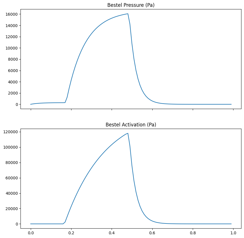
We use the Bestel model from circulation to generate time-dependent profiles for:
Pressure: To load the ventricle.
Activation: To drive active contraction.
We solve the ODEs for the Bestel model first to get the full time traces.
dt = 0.01
times = np.arange(0.0, 1.0, dt)
# Solve Pressure ODE
pressure_model = circulation.bestel.BestelPressure()
res_p = solve_ivp(
    pressure_model,
    [0.0, 1.0],
    [0.0],
    t_eval=times,
    method="Radau",
)
pressure_trace = res_p.y[0] # Pa
                    INFO     INFO:circulation.bestel:                                                                                                                                      bestel.py:177
                              Bestel pressure model
                                    parameters
                             ┏━━━━━━━━━━━━┳━━━━━━━━━┓
                             ┃ Parameter  ┃ Value   ┃
                             ┡━━━━━━━━━━━━╇━━━━━━━━━┩
                             │ t_sys_pre  │ 0.17    │
                             │ t_dias_pre │ 0.484   │
                             │ gamma      │ 0.005   │
                             │ a_max      │ 5.0     │
                             │ a_min      │ -30.0   │
                             │ alpha_pre  │ 5.0     │
                             │ alpha_mid  │ 1.0     │
                             │ sigma_pre  │ 7000.0  │
                             │ sigma_mid  │ 16000.0 │
                             └────────────┴─────────┘
# Solve Activation ODE
activation_model = circulation.bestel.BestelActivation()
res_a = solve_ivp(
    activation_model,
    [0.0, 1.0],
    [0.0],
    t_eval=times,
    method="Radau",
)
activation_trace = res_a.y[0] # Pa
# Plot the input traces
fig, ax = plt.subplots(2, 1, sharex=True, figsize=(10, 10))
ax[0].plot(times, pressure_trace)
ax[0].set_title("Bestel Pressure (Pa)")
ax[1].plot(times, activation_trace)
ax[1].set_title("Bestel Activation (Pa)")
fig.savefig(outdir / "pressure_activation.png")
Mechanics Loop#
We loop over the time steps, updating the pressure and activation in the mechanics model, and solving for the displacement.
# Prepare IO for displacement
vtx = dolfinx.io.VTXWriter(
    geometry.mesh.comm, f"{outdir}/displacement.bp", [problem.u], engine="BP4",
)
vtx.write(0.0)
Setup for regional analysis We define geometric locators to separate the “Curved” free wall from the “Flat” septum. This allows us to compute regional stresses and strains.
def region_curved_locator(x):
    # Logic to identify the curved free wall region
    return np.logical_and(
        np.logical_and(
            np.logical_and(
                np.logical_and(x[0] < -r_inner / 2, np.abs(x[2]) < 3 * height / 4),
                np.abs(x[2]) > height / 4,
            ),
            x[1] < r_inner,
        ),
        x[1] > -r_inner,
    )
def region_flat_locator(x):
    # Logic to identify the flat septum region
    return np.logical_and(
        np.logical_and(
            np.logical_and(
                np.logical_and(x[0] > inner_flat_face_distance / 2, np.abs(x[2]) < 3 * height / 4),
                np.abs(x[2]) > height / 4,
            ),
            x[1] < r_inner,
        ),
        x[1] > -r_inner,
    )
# Create tags for these regions for post-processing integration
cells_curved = dolfinx.mesh.locate_entities(geometry.mesh, 3, region_curved_locator)
cells_flat = dolfinx.mesh.locate_entities(geometry.mesh, 3, region_flat_locator)
curved_marker = 1
flat_marker = 2
marked_values = np.hstack(
    [
        np.full_like(cells_curved, curved_marker),
        np.full_like(cells_flat, flat_marker),
    ],
)
marked_cells = np.hstack([cells_curved, cells_flat])
sorted_idx = np.argsort(marked_cells)
region_tags = dolfinx.mesh.meshtags(
    geometry.mesh,
    geometry.mesh.topology.dim,
    marked_cells[sorted_idx],
    marked_values[sorted_idx],
)
try:
    import pyvista
except ImportError:
    print("Pyvista is not installed")
else:
    # Create plotter and pyvista grid
    p = pyvista.Plotter()
    vtk_mesh = dolfinx.plot.vtk_mesh(geometry.mesh)
    grid = pyvista.UnstructuredGrid(*vtk_mesh)
    grid["regions"] = np.zeros(geometry.mesh.topology.index_map(3).size_local)
    grid["regions"][region_tags.indices] = region_tags.values
    # Attach vector values to grid and warp grid by vector
    actor_0 = p.add_mesh(grid, show_edges=True)

    p.show_axes()
    if not pyvista.OFF_SCREEN:
        p.show()
    else:
        figure_as_array = p.screenshot(outdir / "d_cylinder_cells.png")
# Create integration measure for regions
dx_regions = ufl.Measure("dx", domain=geometry.mesh, subdomain_data=region_tags)
Define forms for stress and strain calculation We compute:
Fiber Stress: sigma_ff = f0 . sigma . f0
Radial Stress: sigma_rr = n0 . sigma . n0
Fiber Strain: E_ff = f0 . E . f0
Radial Strain: E_rr = n0 . E . n0
W = dolfinx.fem.functionspace(geometry.mesh, ("DG", 1))
F_expr = ufl.variable(ufl.grad(problem.u) + ufl.Identity(3))
E_expr = 0.5 * (F_expr.T * F_expr - ufl.Identity(3))
sigma_expr = material.sigma(F_expr) + active_model.S(F_expr.T*F_expr) # Total stress (Active + Passive) approximation
[2025-12-15 07:17:35.919] [info] Checking required entities per dimension
[2025-12-15 07:17:35.919] [info] Cell type: 0 dofmap: 852x4
[2025-12-15 07:17:35.919] [info] Global index computation
[2025-12-15 07:17:35.919] [info] Got 1 index_maps
[2025-12-15 07:17:35.919] [info] Get global indices
fiber_stress = dolfinx.fem.Function(W, name="fiber_stress")
fiber_stress_expr = dolfinx.fem.Expression(
    ufl.inner(sigma_expr * geo.f0, geo.f0),
    W.element.interpolation_points,
)
radial_stress = dolfinx.fem.Function(W, name="radial_stress")
radial_stress_expr = dolfinx.fem.Expression(
    ufl.inner(sigma_expr * geo.n0, geo.n0),
    W.element.interpolation_points,
)
fiber_strain = dolfinx.fem.Function(W, name="fiber_strain")
fiber_strain_expr = dolfinx.fem.Expression(
    ufl.inner(E_expr * geo.f0, geo.f0),
    W.element.interpolation_points,
)
radial_strain = dolfinx.fem.Function(W, name="radial_strain")
radial_strain_expr = dolfinx.fem.Expression(
    ufl.inner(E_expr * geo.n0, geo.n0),
    W.element.interpolation_points,
)
# Setup VTX writer for stress/strain fields
vtx_stress_strain = dolfinx.io.VTXWriter(
    geometry.mesh.comm,
    f"{outdir}/stress_strain.bp",
    [fiber_stress, fiber_strain, radial_stress, radial_strain],
    engine="BP4",
)
vtx_stress_strain.write(0.0)
# Pre-assemble volume forms for averaging
vol_form_flat = dolfinx.fem.form(dolfinx.fem.Constant(geometry.mesh, 1.0) * dx_regions(flat_marker))
vol_form_curved = dolfinx.fem.form(dolfinx.fem.Constant(geometry.mesh, 1.0) * dx_regions(curved_marker))
volume_flat = comm.allreduce(dolfinx.fem.assemble_scalar(vol_form_flat), op=MPI.SUM)
volume_curved = comm.allreduce(dolfinx.fem.assemble_scalar(vol_form_curved), op=MPI.SUM)
# Initialize lists to store time histories
results: dict[str, list[float]] = {
    "fiber_stress_flat": [], "fiber_stress_curved": [],
    "radial_stress_flat": [], "radial_stress_curved": [],
    "fiber_strain_flat": [], "fiber_strain_curved": [],
    "radial_strain_flat": [], "radial_strain_curved": [],
}
# Forms for regional averages
forms = {
    "fiber_stress_flat": dolfinx.fem.form(fiber_stress * dx_regions(flat_marker)),
    "fiber_stress_curved": dolfinx.fem.form(fiber_stress * dx_regions(curved_marker)),
    "radial_stress_flat": dolfinx.fem.form(radial_stress * dx_regions(flat_marker)),
    "radial_stress_curved": dolfinx.fem.form(radial_stress * dx_regions(curved_marker)),
    "fiber_strain_flat": dolfinx.fem.form(fiber_strain * dx_regions(flat_marker)),
    "fiber_strain_curved": dolfinx.fem.form(fiber_strain * dx_regions(curved_marker)),
    "radial_strain_flat": dolfinx.fem.form(radial_strain * dx_regions(flat_marker)),
    "radial_strain_curved": dolfinx.fem.form(radial_strain * dx_regions(curved_marker)),
}
# Run the time loop
for i, (tai, pi, ti) in enumerate(zip(activation_trace, pressure_trace, times)):
    print(f"Step {i}: Time {ti:.3f}, P {pi:.1f}, Ta {tai:.1f}")

    # Update BCs and Activation
    traction.assign(pi)
    Ta.assign(tai)

    # Solve Mechanics
    problem.solve()

    # Post-process fields
    fiber_strain.interpolate(fiber_strain_expr)
    fiber_stress.interpolate(fiber_stress_expr)
    radial_strain.interpolate(radial_strain_expr)
    radial_stress.interpolate(radial_stress_expr)

    # Compute regional averages
    for key in results:
        vol = volume_flat if "flat" in key else volume_curved
        val = comm.allreduce(dolfinx.fem.assemble_scalar(forms[key]), op=MPI.SUM) / vol
        results[key].append(val)

    # Write to file
    vtx.write(ti)
    vtx_stress_strain.write(ti)
    if os.getenv("CI"):
        break
Step 0: Time 0.000, P 0.0, Ta 0.0
[12/15/25 07:17:38] INFO INFO:scifem.solvers:Newton iteration 1: r (abs) = 2.988139062286083e-12 (tol=1e-06), r (rel) = 2.988139062286083e-06 (tol=1e-10) solvers.py:279
6. Plotting Results#
Plot the regional averages of stress and strain over time.
if comm.rank == 0 and not os.getenv("CI"):
    fig, ax = plt.subplots(2, 3, figsize=(15, 10), sharex=True)

    # Row 1: Fiber mechanics
    ax[0, 0].plot(times, results["fiber_stress_flat"], label="Flat")
    ax[0, 0].plot(times, results["fiber_stress_curved"], label="Curved")
    ax[0, 0].set_title("Fiber Stress [Pa]")
    ax[0, 0].legend()

    ax[0, 1].plot(times, results["fiber_strain_flat"], label="Flat")
    ax[0, 1].plot(times, results["fiber_strain_curved"], label="Curved")
    ax[0, 1].set_title("Fiber Strain [-]")

    # Row 2: Radial mechanics
    ax[1, 0].plot(times, results["radial_stress_flat"], label="Flat")
    ax[1, 0].plot(times, results["radial_stress_curved"], label="Curved")
    ax[1, 0].set_title("Radial Stress [Pa]")

    ax[1, 1].plot(times, results["radial_strain_flat"], label="Flat")
    ax[1, 1].plot(times, results["radial_strain_curved"], label="Curved")
    ax[1, 1].set_title("Radial Strain [-]")

    # Loading conditions for reference
    ax[0, 2].plot(times, pressure_trace, 'k--')
    ax[0, 2].set_title("Pressure Load [Pa]")

    ax[1, 2].plot(times, activation_trace, 'r--')
    ax[1, 2].set_title("Activation [Pa]")

    for a in ax.flat:
        a.grid(True)
        a.set_xlabel("Time [s]")

    fig.tight_layout()
    fig.savefig(outdir / "stress_strain_analysis.png")
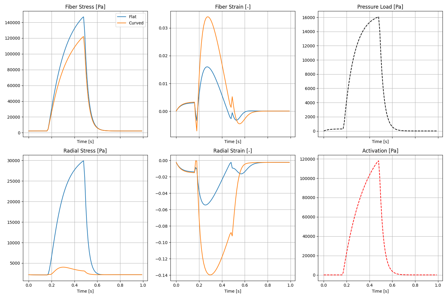
Fig. 3 Stress and strain in the cylinder over time.#