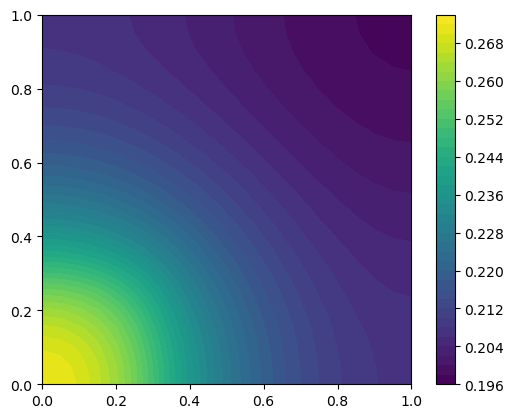
Diffusion in a square domain with a stimulus in the lower left corner#
This demo solves the monodomain equation on a square domain with a stimulus in the lower left corner. The stimulus is defined as a constant value in a subdomain.
import beat
import dolfin
import matplotlib.pyplot as plt
mesh = dolfin.UnitSquareMesh(20, 20)
S = dolfin.Constant(1.0)
S1_subdomain = dolfin.CompiledSubDomain(
    "x[0] <= L + DOLFIN_EPS && x[1] <= L + DOLFIN_EPS",
    L=0.3,
)
S1_markers = dolfin.MeshFunction("size_t", mesh, 2)
S1_marker = 1
S1_subdomain.mark(S1_markers, S1_marker)
I_s = beat.base_model.Stimulus(
    expr=S, dz=dolfin.dx(domain=mesh, subdomain_data=S1_markers)(S1_marker)
)
time = dolfin.Constant(0.0)
model = beat.MonodomainModel(time=time, mesh=mesh, M=1.0, I_s=I_s)
res = model.solve((0, 2.5), dt=0.1)
Calling FFC just-in-time (JIT) compiler, this may take some time.
Calling FFC just-in-time (JIT) compiler, this may take some time.
Calling FFC just-in-time (JIT) compiler, this may take some time.
Calling FFC just-in-time (JIT) compiler, this may take some time.
Calling FFC just-in-time (JIT) compiler, this may take some time.
Calling FFC just-in-time (JIT) compiler, this may take some time.
Calling FFC just-in-time (JIT) compiler, this may take some time.
Calling FFC just-in-time (JIT) compiler, this may take some time.
Calling FFC just-in-time (JIT) compiler, this may take some time.
fig = plt.figure()
im = dolfin.plot(res.state)
fig.colorbar(im)
fig.savefig("diffusion.png")