Endocardial stimulation#
In this demo we show how to load an ODE file and use it to simulate endocardial stimulation.

Fig. 1 Electrode positions#
from collections import defaultdict
from pathlib import Path
import cardiac_geometries
import numpy as np
import matplotlib.pyplot as plt
import dolfin
import pyvista


try:
    from tqdm import tqdm
except ImportError:
    tqdm = lambda x: x

import beat
import beat.viz
import gotranx
def get_data(datadir="data_endocardial_stimulation"):
    datadir = Path(datadir)
    msh_file = datadir / "biv_ellipsoid.msh"
    if not msh_file.is_file():
        cardiac_geometries.create_biv_ellipsoid(
            datadir,
            char_length=0.2,  # Reduce this value to get a finer mesh
            center_lv_y=0.2,
            center_lv_z=0.0,
            a_endo_lv=5.0,
            b_endo_lv=2.2,
            c_endo_lv=2.2,
            a_epi_lv=6.0,
            b_epi_lv=3.0,
            c_epi_lv=3.0,
            center_rv_y=1.0,
            center_rv_z=0.0,
            a_endo_rv=6.0,
            b_endo_rv=2.5,
            c_endo_rv=2.7,
            a_epi_rv=8.0,
            b_epi_rv=5.5,
            c_epi_rv=4.0,
            create_fibers=True,
        )

    return cardiac_geometries.geometry.Geometry.from_folder(datadir)
def load_from_file(heart_mesh, xdmffile, key="v", stop_index=None):
    V = dolfin.FunctionSpace(heart_mesh, "Lagrange", 1)
    v = dolfin.Function(V)

    timesteps = beat.postprocess.load_timesteps_from_xdmf(xdmffile)
    with dolfin.XDMFFile(Path(xdmffile).as_posix()) as f:
        for i, t in tqdm(timesteps.items()):
            f.read_checkpoint(v, key, i)
            yield v.copy(deepcopy=True), t
def compute_ecg_recovery():
    datadir = Path("data_endocardial_stimulation")
    xdmffile = datadir / "state.xdmf"
    data = get_data(datadir=datadir)

    # https://litfl.com/ecg-lead-positioning/
    vs = load_from_file(data.mesh, xdmffile, key="V")

    leads = dict(
        RA=(-15.0, 0.0, -10.0),
        LA=(4.0, -12.0, -7.0),
        RL=(0.0, 20.0, 3.0),
        LL=(17.0, 11.0, 7.0),
        V1=(-3.0, 4.0, -9.0),
        V2=(0.0, 2.0, -8.0),
        V3=(3.0, 1.0, -8.0),
        V4=(6.0, 1.0, -6.0),
        V5=(10.0, 2.0, 0.0),
        V6=(10.0, -6.0, 2.0),
    )

    fname = datadir / "extracellular_potential.npy"
    if not fname.is_file():
        phie = defaultdict(list)
        time = []
        for v, t in vs:
            time.append(t)
            for name, point in leads.items():
                phie[name].append(
                    beat.ecg.ecg_recovery(v=v, mesh=data.mesh, sigma_b=1.0, point=point)
                )
        np.save(fname, {"phie": phie, "time": time})

    phie_time = np.load(fname, allow_pickle=True).item()
    phie = phie_time["phie"]
    time = phie_time["time"]

    fig, ax = plt.subplots(2, 5, sharex=True, figsize=(12, 8))
    for i, (name, values) in enumerate(phie.items()):
        axi = ax.flatten()[i]
        axi.plot(time, values)
        axi.set_title(name)
    fig.savefig(datadir / "extracellular_potential.png")

    ecg = beat.ecg.Leads12(**{k: np.array(v) for k, v in phie.items()})
    fig, ax = plt.subplots(3, 4, sharex=True, figsize=(12, 8))
    for i, name in enumerate(
        [
            "I",
            "II",
            "III",
            "aVR",
            "aVL",
            "aVF",
            "V1_",
            "V2_",
            "V3_",
            "V4_",
            "V5_",
            "V6_",
        ]
    ):
        y = getattr(ecg, name)
        axi = ax.flatten()[i]
        axi.plot(time, y)
        axi.set_title(name)
    fig.savefig(datadir / "ecg_12_leads.png")
here = Path.cwd()
datadir = here / "data_endocardial_stimulation"
model_path = Path("ORdmm_Land.py")
if not model_path.is_file():
    ode = gotranx.load_ode(here / ".." / "odes" / "ORdmm_Land.ode")
    code = gotranx.cli.gotran2py.get_code(
        ode, scheme=[gotranx.schemes.Scheme.forward_generalized_rush_larsen]
    )
    model_path.write_text(code)
2026-01-18 21:31:54 [info ] Load ode /__w/fenics-beat/fenics-beat/demos/../odes/ORdmm_Land.ode
2026-01-18 21:31:55 [info ] Num states 48
2026-01-18 21:31:55 [info ] Num parameters 139
import ORdmm_Land
model = ORdmm_Land.__dict__
data = get_data(datadir=datadir)
Calculating scalar fields
Compute scalar laplacian solutions with the markers:
base: [1]
lv: [2]
rv: [3]
epi: [4]
  Num vertices: 29407
  Num cells: 139200
Calling FFC just-in-time (JIT) compiler, this may take some time.
Calling FFC just-in-time (JIT) compiler, this may take some time.
Calling FFC just-in-time (JIT) compiler, this may take some time.
Calling FFC just-in-time (JIT) compiler, this may take some time.
Calling FFC just-in-time (JIT) compiler, this may take some time.
Calling FFC just-in-time (JIT) compiler, this may take some time.
Calling FFC just-in-time (JIT) compiler, this may take some time.
Apex coord: (7.96, 1.72, -0.05)
Solving Laplace equation
 lv = 1, rv, epi = 0
 rv = 1, lv, epi = 0
 epi = 1, lv, rv = 0

Calculating gradients
Calling FFC just-in-time (JIT) compiler, this may take some time.
Calling FFC just-in-time (JIT) compiler, this may take some time.
Calling FFC just-in-time (JIT) compiler, this may take some time.
Calling FFC just-in-time (JIT) compiler, this may take some time.
Calling FFC just-in-time (JIT) compiler, this may take some time.
Compute fiber-sheet system
Angles:
alpha:
 endo_lv: -60
 epi_lv: 60
 endo_septum: -60
 epi_septum: 60
 endo_rv: -60
 epi_rv: 60
beta:
 endo_lv: -65
 epi_lv: 25
 endo_septum: -65
 epi_septum: 25
 endo_rv: -65
 epi_rv: 25
mesh_unit = "mm"
V = dolfin.FunctionSpace(data.mesh, "Lagrange", 1)

markers = beat.utils.expand_layer_biv(
    V=V,
    mfun=data.ffun,
    endo_lv_marker=data.markers["ENDO_LV"][0],
    endo_rv_marker=data.markers["ENDO_RV"][0],
    epi_marker=data.markers["EPI"][0],
    endo_size=0.3,
    epi_size=0.3,
)


pyvista.start_xvfb()
plotter_markers = pyvista.Plotter()
topology, cell_types, x = beat.viz.create_vtk_structures(V)
grid = pyvista.UnstructuredGrid(topology, cell_types, x)
grid["markers"] = markers.vector().get_local()
plotter_markers.add_mesh(grid, show_edges=True)
/usr/lib/python3/dist-packages/pyvista/plotting/utilities/xvfb.py:48: PyVistaDeprecationWarning: This function is deprecated and will be removed in future version of PyVista. Use vtk-osmesa instead.
  warnings.warn(
Actor (0x7f6ab2306020)
  Center:                     (3.998753816684164, 1.199999999999994, 0.0)
  Pickable:                   True
  Position:                   (0.0, 0.0, 0.0)
  Scale:                      (1.0, 1.0, 1.0)
  Visible:                    True
  X Bounds                    0.000E+00, 7.998E+00
  Y Bounds                    -4.300E+00, 6.700E+00
  Z Bounds                    -4.000E+00, 4.000E+00
  User matrix:                Identity
  Has mapper:                 True

Property (0x7f6ab23064a0)
  Ambient:                     0.0
  Ambient color:               Color(name='lightblue', hex='#add8e6ff', opacity=255)
  Anisotropy:                  0.0
  Color:                       Color(name='lightblue', hex='#add8e6ff', opacity=255)
  Culling:                     "none"
  Diffuse:                     1.0
  Diffuse color:               Color(name='lightblue', hex='#add8e6ff', opacity=255)
  Edge color:                  Color(name='black', hex='#000000ff', opacity=255)
  Edge opacity:                1.0
  Interpolation:               0
  Lighting:                    True
  Line width:                  1.0
  Metallic:                    0.0
  Opacity:                     1.0
  Point size:                  5.0
  Render lines as tubes:       False
  Render points as spheres:    False
  Roughness:                   0.5
  Show edges:                  True
  Specular:                    0.0
  Specular color:              Color(name='lightblue', hex='#add8e6ff', opacity=255)
  Specular power:              100.0
  Style:                       "Surface"

DataSetMapper (0x7f6ab2305d20)
  Scalar visibility:           True
  Scalar range:                (0.0, 2.0)
  Interpolate before mapping:  True
  Scalar map mode:             point
  Color mode:                  map

Attached dataset:
UnstructuredGrid (0x7f6ab2305c60)
  N Cells:    139200
  N Points:   29407
  X Bounds:   0.000e+00, 7.998e+00
  Y Bounds:   -4.300e+00, 6.700e+00
  Z Bounds:   -4.000e+00, 4.000e+00
  N Arrays:   1
plotter_markers.view_zy()
plotter_markers.camera.zoom(4)
if not pyvista.OFF_SCREEN:
    plotter_markers.show()
else:
    figure = plotter_markers.screenshot("fundamentals_mesh.png")
init_states = {
    0: model["init_state_values"](),
    1: model["init_state_values"](),
    2: model["init_state_values"](),
}
# endo = 0, epi = 1, M = 2
parameters = {
    0: model["init_parameter_values"](amp=0.0, celltype=2),
    1: model["init_parameter_values"](amp=0.0, celltype=0),
    2: model["init_parameter_values"](amp=0.0, celltype=1),
}
fun = {
    0: model["forward_generalized_rush_larsen"],
    1: model["forward_generalized_rush_larsen"],
    2: model["forward_generalized_rush_larsen"],
}
v_index = {
    0: model["state_index"]("v"),
    1: model["state_index"]("v"),
    2: model["state_index"]("v"),
}

# Surface to volume ratio
chi = 140.0 * beat.units.ureg("mm**-1")
# Membrane capacitance
C_m = 0.01 * beat.units.ureg("uF/mm**2")

time = dolfin.Constant(0.0)

subdomain_data = dolfin.MeshFunction("size_t", data.mesh, 2)
subdomain_data.set_all(0)
marker = 1
subdomain_data.array()[data.ffun.array() == data.markers["ENDO_LV"][0]] = 1
subdomain_data.array()[data.ffun.array() == data.markers["ENDO_RV"][0]] = 1
I_s = beat.stimulation.define_stimulus(
    mesh=data.mesh,
    chi=chi,
    mesh_unit=mesh_unit,
    time=time,
    subdomain_data=subdomain_data,
    marker=marker,
    amplitude=500.0,
)

M = beat.conductivities.define_conductivity_tensor(
    chi=chi, f0=data.f0, g_il=0.17, g_it=0.019, g_el=0.62, g_et=0.24
)

params = {"preconditioner": "sor", "use_custom_preconditioner": False}
pde = beat.MonodomainModel(
    time=time,
    C_m=C_m.to(f"uF/{mesh_unit}**2").magnitude,
    mesh=data.mesh,
    M=M,
    I_s=I_s,
    params=params,
)

ode = beat.odesolver.DolfinMultiODESolver(
    v_ode=dolfin.Function(V),
    v_pde=pde.state,
    markers=markers,
    num_states={i: len(s) for i, s in init_states.items()},
    fun=fun,
    init_states=init_states,
    parameters=parameters,
    v_index=v_index,
)
Calling FFC just-in-time (JIT) compiler, this may take some time.
Calling FFC just-in-time (JIT) compiler, this may take some time.
Calling FFC just-in-time (JIT) compiler, this may take some time.
T = 1
# Change to 500 to simulate the full cardiac cycle
# T = 500
t = 0.0
dt = 0.05
solver = beat.MonodomainSplittingSolver(pde=pde, ode=ode)

fname = (datadir / "state.xdmf").as_posix()
i = 0
while t < T + 1e-12:
    if i % 20 == 0:
        v = solver.pde.state.vector().get_local()
        print(f"Solve for {t=:.2f}, {v.max() =}, {v.min() = }")
        with dolfin.XDMFFile(dolfin.MPI.comm_world, fname) as xdmf:
            xdmf.parameters["functions_share_mesh"] = True
            xdmf.parameters["rewrite_function_mesh"] = False
            xdmf.write_checkpoint(
                solver.pde.state,
                "V",
                float(t),
                dolfin.XDMFFile.Encoding.HDF5,
                True,
            )
    solver.step((t, t + dt))
    i += 1
    t += dt
Calling FFC just-in-time (JIT) compiler, this may take some time.
Calling FFC just-in-time (JIT) compiler, this may take some time.
Solve for t=0.00, v.max() =-86.99999999999982, v.min() = -87.00000000000011
Calling FFC just-in-time (JIT) compiler, this may take some time.
Calling FFC just-in-time (JIT) compiler, this may take some time.
Calling FFC just-in-time (JIT) compiler, this may take some time.
Calling FFC just-in-time (JIT) compiler, this may take some time.
Solve for t=1.00, v.max() =-49.02179661083312, v.min() = -91.9007132725155
compute_ecg_recovery()
0%| | 0/2 [00:00<?, ?it/s]
Calling FFC just-in-time (JIT) compiler, this may take some time.
Calling FFC just-in-time (JIT) compiler, this may take some time.
50%|█████ | 1/2 [00:01<00:01, 1.66s/it]
100%|██████████| 2/2 [00:02<00:00, 1.21s/it]
100%|██████████| 2/2 [00:02<00:00, 1.28s/it]


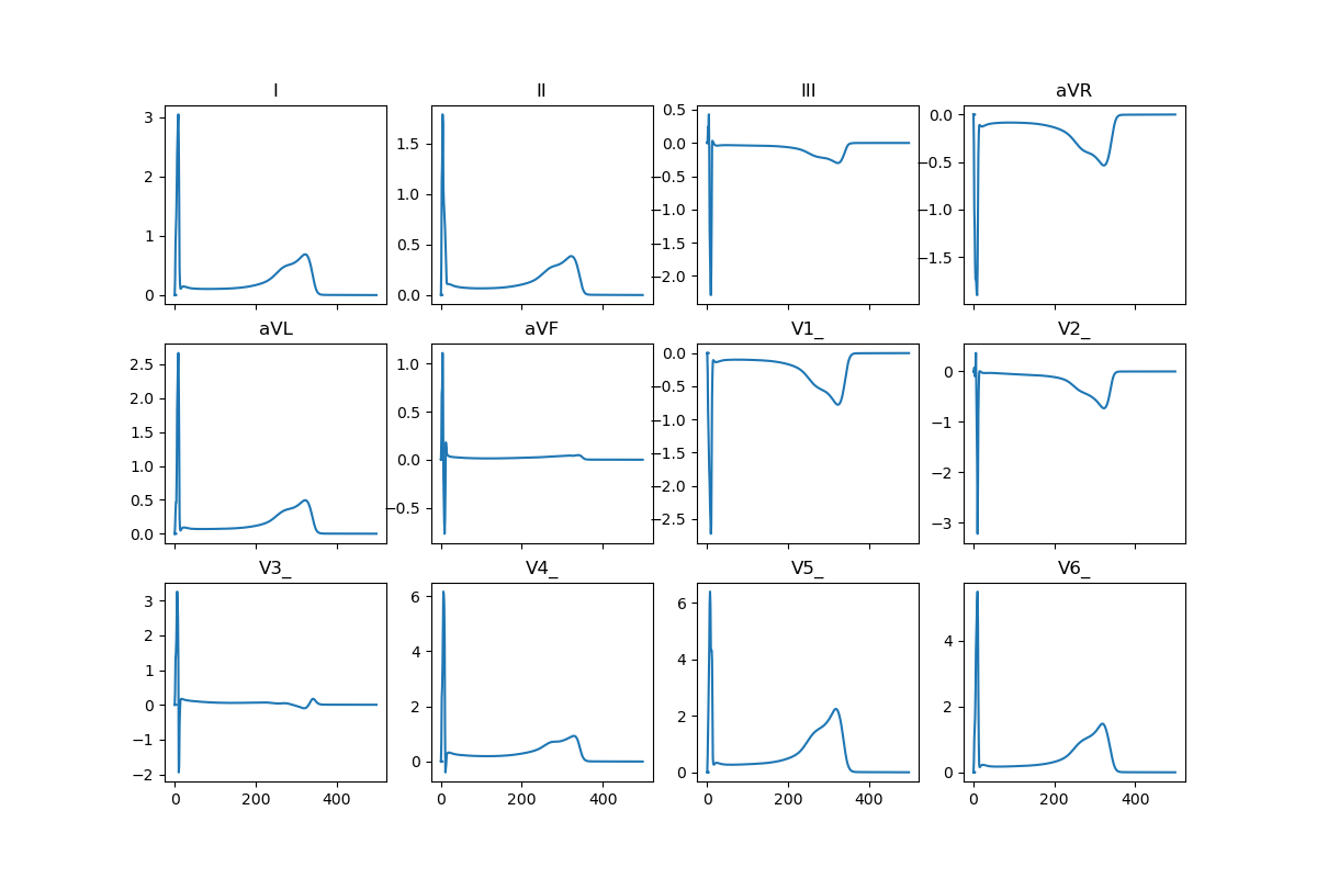
Fig. 2 Precomputed 12-lead ECG#