Complete Multiscale Simulation with Prestressing#
This comprehensive demo illustrates a complete cardiac mechanics pipeline involving:
Geometry: Generating a Bi-Ventricular (BiV) mesh from the UK Biobank Atlas, rotating it, and generating fiber fields using LDRB, which is similar to what is implemented in rotated BiV demo. In addition we show how to generate additional fields such as longitudinal and circumferential fields for computing e.g longitudinal strain, similar to the additional data demo in
caridac-geometriesx0D Circulation: Running a 0D closed-loop circulation model (Regazzoni) to establish physiological pressure traces.
Prestressing: Solving the Inverse Elasticity Problem (IEP) to find the unloaded reference configuration that matches the atlas geometry at End-Diastole (ED). This is similar to what is impemtented in the BiV prestress demo
Inflation: Ramping the unloaded mesh back to the End-Diastolic state to initialize the dynamic simulation.
Multiscale Coupling: Running a forward simulation coupled to the 0D circulation model, which is similar to what is implemented in the time dependent BiV problem
Post-processing: Computing Fiber Stress and Fiber Strain.
Imports and Setup#
import json
import os
import logging
import shutil
from pathlib import Path
from mpi4py import MPI
import numpy as np
import matplotlib.pyplot as plt
from matplotlib.gridspec import GridSpec
import dolfinx
import ufl
import ldrb
import io4dolfinx
# Cardiac specific libraries
import cardiac_geometries
import cardiac_geometries.geometry
import circulation
from circulation.regazzoni2020 import Regazzoni2020
import pulse
# Helper function to convert units
def mmHg_to_kPa(x):
    return x * 0.133322
# JSON serializer for numpy types
def custom_json(obj):
    if isinstance(obj, np.float64):
        return float(obj)
    elif isinstance(obj, np.ndarray):
        return obj.tolist()
    else:
        return str(obj)
# Setup logging to print only from rank 0
class MPIFilter(logging.Filter):
    def __init__(self, comm, *args, **kwargs):
        super().__init__(*args, **kwargs)
        self.comm = comm

    def filter(self, record):
        return 1 if self.comm.rank == 0 else 0
outdir = Path("results_biv_complete_cycle")
outdir.mkdir(parents=True, exist_ok=True)
geodir = outdir / "geometry"
circulation.log.setup_logging(logging.INFO)
logger = logging.getLogger("pulse")
scifem_logger = logging.getLogger("scifem")
scifem_logger.setLevel(logging.WARNING)
comm = MPI.COMM_WORLD
mpi_filter = MPIFilter(comm)
logger.addFilter(mpi_filter)
Geometry Generation & Rotation#
We generate the BiV geometry from the UK Biobank Atlas, rotate it to align the base normal with the x-axis, and generate fiber fields using LDRB. The fibers are based on the fiber orientation angles from https://doi.org/10.1002/cnm.3185. Additional data such as fibers in DG 1 space are also stored for post-processing. This is useful if we want to compute stress/strain at intermediate points later on. The fibers used for the mechanics simulation are in a quadrature space to avoid interpolation errors.
if not (geodir / "geometry.bp").exists():
    logger.info("Generating and processing geometry...")
    mode = -1
    std = 0
    char_length = 10.0

    geo = cardiac_geometries.mesh.ukb(
        outdir=geodir,
        comm=comm,
        mode=mode,
        std=std,
        case="ED",
        char_length_max=char_length,
        char_length_min=char_length,
        clipped=True,
    )

    # Rotate Mesh (Base Normal -> X-axis)
    geo = geo.rotate(target_normal=[1.0, 0.0, 0.0], base_marker="BASE")

    fiber_angles = dict(
        alpha_endo_lv=60,
        alpha_epi_lv=-60,
        alpha_endo_rv=90,
        alpha_epi_rv=-25,
        beta_endo_lv=-20,
        beta_epi_lv=20,
        beta_endo_rv=0,
        beta_epi_rv=20,
    )

    # Generate Fibers (LDRB)
    system = ldrb.dolfinx_ldrb(
        mesh=geo.mesh,
        ffun=geo.ffun,
        markers=cardiac_geometries.mesh.transform_markers(geo.markers, clipped=True),
        **fiber_angles,
        fiber_space="Quadrature_6",
    )

    # Additional Vectors for Analysis in DG 1 Space for computing stress/strain later
    fiber_space = "DG_1"
    system_fibers = ldrb.dolfinx_ldrb(
        mesh=geo.mesh,
        ffun=geo.ffun,
        markers=cardiac_geometries.mesh.transform_markers(geo.markers, clipped=True),
        **fiber_angles,
        fiber_space=fiber_space,
    )

    # Save Everything
    additional_data = {
        "f0_DG_1": system_fibers.f0,
        "s0_DG_1": system_fibers.s0,
        "n0_DG_1": system_fibers.n0,
    }

    if (geodir / "geometry.bp").exists():
        shutil.rmtree(geodir / "geometry.bp")

    cardiac_geometries.geometry.save_geometry(
        path=geodir / "geometry.bp",
        mesh=geo.mesh,
        ffun=geo.ffun,
        markers=geo.markers,
        info=geo.info,
        f0=system.f0,
        s0=system.s0,
        n0=system.n0,
        additional_data=additional_data,
    )
[06/30/26 21:16:44] INFO INFO:pulse:Generating and processing geometry... 8419240.py:2
INFO INFO:ukb.surface:Saved results_biv_complete_cycle/geometry/EPI_ED.stl surface.py:201
INFO INFO:ukb.surface:Saved results_biv_complete_cycle/geometry/MV_ED.stl surface.py:206
INFO INFO:ukb.surface:Saved results_biv_complete_cycle/geometry/AV_ED.stl surface.py:206
INFO INFO:ukb.surface:Saved results_biv_complete_cycle/geometry/TV_ED.stl surface.py:206
INFO INFO:ukb.surface:Saved results_biv_complete_cycle/geometry/PV_ED.stl surface.py:206
INFO INFO:ukb.surface:Saved results_biv_complete_cycle/geometry/LV_ED.stl surface.py:214
INFO INFO:ukb.surface:Saved results_biv_complete_cycle/geometry/RV_ED.stl surface.py:214
INFO INFO:ukb.surface:Saved results_biv_complete_cycle/geometry/RVFW_ED.stl surface.py:214
[06/30/26 21:16:45] INFO INFO:ukb.clip:Reading results_biv_complete_cycle/geometry/LV_ED.stl clip.py:163
Warning: PLY writer doesn't support multidimensional point data yet. Skipping Normals.
Warning: PLY doesn't support 64-bit integers. Casting down to 32-bit.
Warning: PLY writer doesn't support multidimensional point data yet. Skipping Normals.
Warning: PLY doesn't support 64-bit integers. Casting down to 32-bit.
Warning: PLY writer doesn't support multidimensional point data yet. Skipping Normals.
Warning: PLY doesn't support 64-bit integers. Casting down to 32-bit.
0
INFO INFO:ukb.mesh:Creating clipped mesh for ED with char_length_max=10.0, char_length_min=10.0 mesh.py:264
2026-06-30 21:16:45 [debug ] Convert file results_biv_complete_cycle/geometry/ED_clipped.msh to dolfin
Info    : Reading 'results_biv_complete_cycle/geometry/ED_clipped.msh'...
Info    : 11 entities
Info    : 707 nodes
Info    : 3494 elements
Info    : 3 parametrizations
Info    : [  0%] Processing parametrizations
Info    : [ 10%] Processing parametrizations
Info    : [ 40%] Processing parametrizations
Info    : Done reading 'results_biv_complete_cycle/geometry/ED_clipped.msh'
                    INFO     INFO:ldrb.ldrb:Compute scalar laplacian solutions with the markers:                                                                                             ldrb.py:619
                             lv: [1]
                             rv: [2]
                             epi: [3]
                             base: [4]
                    INFO     INFO:ldrb.ldrb:alpha:                                                                                                                                            ldrb.py:86
                              endo_lv: 60
                              epi_lv: -60
                              endo_septum: 60
                              epi_septum: -60
                              endo_rv: 60
                              epi_rv: -60
                    INFO     INFO:ldrb.ldrb:beta:                                                                                                                                             ldrb.py:98
                              endo_lv: 0
                              epi_lv: 0
                              endo_septum: 0
                              epi_septum: 0
                              endo_rv: 0
                              epi_rv: 0
2026-06-30 21:16:47 [debug ] Write f0: f0
2026-06-30 21:16:47 [debug ] Write s0: s0
2026-06-30 21:16:47 [debug ] Write n0: n0
2026-06-30 21:16:47 [debug ] Write lv: f
2026-06-30 21:16:47 [debug ] Write rv: f
2026-06-30 21:16:47 [debug ] Write epi: f
2026-06-30 21:16:47 [debug ] Write lv_rv: f
2026-06-30 21:16:47 [debug ] Write apex: f
2026-06-30 21:16:47 [debug ] Write lv_scalar: f
2026-06-30 21:16:47 [debug ] Write rv_scalar: f
2026-06-30 21:16:47 [debug ] Write epi_scalar: f
2026-06-30 21:16:47 [debug ] Write lv_rv_scalar: f
2026-06-30 21:16:47 [debug ] Write lv_gradient: f
2026-06-30 21:16:47 [debug ] Write rv_gradient: f
2026-06-30 21:16:47 [debug ] Write epi_gradient: f
2026-06-30 21:16:47 [debug ] Write apex_gradient: f
2026-06-30 21:16:47 [debug ] Write markers_scalar: f
2026-06-30 21:16:47 [info ] Rotated geometry. Base normal [-0.71608436 0.54439464 0.43687259] aligned to [1.0, 0.0, 0.0]
2026-06-30 21:16:47 [debug    ] Rotation matrix:
[[-0.71608436  0.54439464  0.43687259]
 [-0.54439464 -0.04385067 -0.83768227]
 [-0.43687259 -0.83768227  0.32776631]]
                    INFO     INFO:ldrb.ldrb:Compute scalar laplacian solutions with the markers:                                                                                             ldrb.py:619
                             lv: [1]
                             rv: [2]
                             epi: [3]
                             base: [4]
                    INFO     INFO:ldrb.ldrb:alpha:                                                                                                                                            ldrb.py:86
                              endo_lv: 60
                              epi_lv: -60
                              endo_septum: 60
                              epi_septum: -60
                              endo_rv: 90
                              epi_rv: -25
                    INFO     INFO:ldrb.ldrb:beta:                                                                                                                                             ldrb.py:98
                              endo_lv: -20
                              epi_lv: 20
                              endo_septum: -20
                              epi_septum: 20
                              endo_rv: -20
                              epi_rv: 20
                    INFO     INFO:ldrb.ldrb:Compute scalar laplacian solutions with the markers:                                                                                             ldrb.py:619
                             lv: [1]
                             rv: [2]
                             epi: [3]
                             base: [4]
We load the generated geometry
geo = cardiac_geometries.geometry.Geometry.from_folder(comm=comm, folder=geodir)
[06/30/26 21:16:48] INFO INFO:cardiac_geometries.geometry:Reading geometry from results_biv_complete_cycle/geometry geometry.py:518
Scale to meters
scale = 1e-3
geo.mesh.geometry.x[:] *= scale
geometry = pulse.HeartGeometry.from_cardiac_geometries(
    geo, metadata={"quadrature_degree": 6},
)
Store Target Volumes (ED)
# Conversion from m3 to mL
volume2ml = 1e6
# Unit of the mesh is now meters
mesh_unit = "m"
Target ED volumes from original mesh
lvv_target = comm.allreduce(geometry.volume("LV"), op=MPI.SUM)
rvv_target = comm.allreduce(geometry.volume("RV"), op=MPI.SUM)
logger.info(
    f"ED Volumes: LV={lvv_target * volume2ml:.2f} mL, RV={rvv_target * volume2ml:.2f} mL",
)
INFO INFO:pulse:ED Volumes: LV=109.15 mL, RV=74.86 mL 2954599161.py:3
0D Circulation Model (Initialization)#
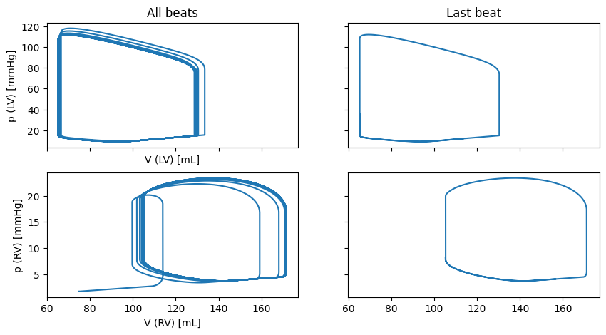
We run the 0D circulation model to get the target End-Diastolic pressures for prestressing.
def run_0D(init_state, nbeats=10):
    logger.info("Running 0D circulation model to steady state...")

    model = Regazzoni2020()
    history = model.solve(num_beats=nbeats, initial_state=init_state)
    state = dict(zip(model.state_names(), model.state))

    return history, state
First use the target ED volumes to initialize the circulation model
init_state_circ = {
    "V_LV": lvv_target * volume2ml * circulation.units.ureg("mL"),
    "V_RV": rvv_target * volume2ml * circulation.units.ureg("mL"),
}
Run to steady state
if comm.rank == 0:
    history, circ_state = run_0D(init_state=init_state_circ)
    np.save(outdir / "state.npy", circ_state, allow_pickle=True)
    np.save(outdir / "history.npy", history, allow_pickle=True)
comm.Barrier()
INFO INFO:pulse:Running 0D circulation model to steady state... 1721694897.py:2
                    INFO     INFO:circulation.base:                                                                                                                                          base.py:134
                                                    Circulation model parameters (Regazzoni2020)
                             ┏━━━━━━━━━━━━━━━━━━━━━━━━━━━━━━━━━━━━━━━┳━━━━━━━━━━━━━━━━━━━━━━━━━━━━━━━━━━━━━━━━━━━━━━━━━┓
                             ┃ Parameter                             ┃ Value                                           ┃
                             ┡━━━━━━━━━━━━━━━━━━━━━━━━━━━━━━━━━━━━━━━╇━━━━━━━━━━━━━━━━━━━━━━━━━━━━━━━━━━━━━━━━━━━━━━━━━┩
                             │ HR                                    │ 1.25 hertz                                      │
                             │ chambers.LA.EA                        │ 0.07 millimeter_Hg / milliliter                 │
                             │ chambers.LA.EB                        │ 0.18 millimeter_Hg / milliliter                 │
                             │ chambers.LA.TC                        │ 0.17 second                                     │
                             │ chambers.LA.TR                        │ 0.17 second                                     │
                             │ chambers.LA.tC                        │ 0.9 second                                      │
                             │ chambers.LA.V0                        │ 4.0 milliliter                                  │
                             │ chambers.LV.EA                        │ 4.482 millimeter_Hg / milliliter                │
                             │ chambers.LV.EB                        │ 0.17 millimeter_Hg / milliliter                 │
                             │ chambers.LV.TC                        │ 0.25 second                                     │
                             │ chambers.LV.TR                        │ 0.4 second                                      │
                             │ chambers.LV.tC                        │ 0.1 second                                      │
                             │ chambers.LV.V0                        │ 42.0 milliliter                                 │
                             │ chambers.RA.EA                        │ 0.06 millimeter_Hg / milliliter                 │
                             │ chambers.RA.EB                        │ 0.07 millimeter_Hg / milliliter                 │
                             │ chambers.RA.TC                        │ 0.17 second                                     │
                             │ chambers.RA.TR                        │ 0.17 second                                     │
                             │ chambers.RA.tC                        │ 0.9 second                                      │
                             │ chambers.RA.V0                        │ 4.0 milliliter                                  │
                             │ chambers.RV.EA                        │ 0.2 millimeter_Hg / milliliter                  │
                             │ chambers.RV.EB                        │ 0.029 millimeter_Hg / milliliter                │
                             │ chambers.RV.TC                        │ 0.25 second                                     │
                             │ chambers.RV.TR                        │ 0.4 second                                      │
                             │ chambers.RV.tC                        │ 0.1 second                                      │
                             │ chambers.RV.V0                        │ 16.0 milliliter                                 │
                             │ valves.MV.Rmin                        │ 0.0075 millimeter_Hg * second / milliliter      │
                             │ valves.MV.Rmax                        │ 75006.2 millimeter_Hg * second / milliliter     │
                             │ valves.AV.Rmin                        │ 0.0075 millimeter_Hg * second / milliliter      │
                             │ valves.AV.Rmax                        │ 75006.2 millimeter_Hg * second / milliliter     │
                             │ valves.TV.Rmin                        │ 0.0075 millimeter_Hg * second / milliliter      │
                             │ valves.TV.Rmax                        │ 75006.2 millimeter_Hg * second / milliliter     │
                             │ valves.PV.Rmin                        │ 0.0075 millimeter_Hg * second / milliliter      │
                             │ valves.PV.Rmax                        │ 75006.2 millimeter_Hg * second / milliliter     │
                             │ circulation.SYS.R_AR                  │ 0.733 millimeter_Hg * second / milliliter       │
                             │ circulation.SYS.C_AR                  │ 1.372 milliliter / millimeter_Hg                │
                             │ circulation.SYS.R_VEN                 │ 0.32 millimeter_Hg * second / milliliter        │
                             │ circulation.SYS.C_VEN                 │ 11.363 milliliter / millimeter_Hg               │
                             │ circulation.SYS.L_AR                  │ 0.005 millimeter_Hg * second ** 2 / milliliter  │
                             │ circulation.SYS.L_VEN                 │ 0.0005 millimeter_Hg * second ** 2 / milliliter │
                             │ circulation.PUL.R_AR                  │ 0.046 millimeter_Hg * second / milliliter       │
                             │ circulation.PUL.C_AR                  │ 20.0 milliliter / millimeter_Hg                 │
                             │ circulation.PUL.R_VEN                 │ 0.0015 millimeter_Hg * second / milliliter      │
                             │ circulation.PUL.C_VEN                 │ 16.0 milliliter / millimeter_Hg                 │
                             │ circulation.PUL.L_AR                  │ 0.0005 millimeter_Hg * second ** 2 / milliliter │
                             │ circulation.PUL.L_VEN                 │ 0.0005 millimeter_Hg * second ** 2 / milliliter │
                             │ circulation.external.start_withdrawal │ 0.0 second                                      │
                             │ circulation.external.end_withdrawal   │ 0.0 second                                      │
                             │ circulation.external.start_infusion   │ 0.0 second                                      │
                             │ circulation.external.end_infusion     │ 0.0 second                                      │
                             │ circulation.external.flow_withdrawal  │ 0.0 milliliter / second                         │
                             │ circulation.external.flow_infusion    │ 0.0 milliliter / second                         │
                             └───────────────────────────────────────┴─────────────────────────────────────────────────┘
                    INFO     INFO:circulation.base:                                                                                                                                          base.py:141
                                  Circulation model initial states
                                           (Regazzoni2020)
                             ┏━━━━━━━━━━━┳━━━━━━━━━━━━━━━━━━━━━━━━━━━━━┓
                             ┃ State     ┃ Value                       ┃
                             ┡━━━━━━━━━━━╇━━━━━━━━━━━━━━━━━━━━━━━━━━━━━┩
                             │ V_LA      │ 87.183 milliliter           │
                             │ V_LV      │ 118.52 milliliter           │
                             │ V_RA      │ 86.833 milliliter           │
                             │ V_RV      │ 166.177 milliliter          │
                             │ p_AR_SYS  │ 87.675 millimeter_Hg        │
                             │ p_VEN_SYS │ 35.898 millimeter_Hg        │
                             │ p_AR_PUL  │ 19.545 millimeter_Hg        │
                             │ p_VEN_PUL │ 15.004 millimeter_Hg        │
                             │ Q_AR_SYS  │ 71.104 milliliter / second  │
                             │ Q_VEN_SYS │ 94.039 milliliter / second  │
                             │ Q_AR_PUL  │ 94.084 milliliter / second  │
                             │ Q_VEN_PUL │ 473.279 milliliter / second │
                             └───────────┴─────────────────────────────┘
Compute errors in volumes at the end of the 0D run
error_LV = circ_state["V_LV"] - init_state_circ["V_LV"].magnitude
error_RV = circ_state["V_RV"] - init_state_circ["V_RV"].magnitude
Let us plot the results from the circulation model
if comm.rank == 0:
    fig, ax = plt.subplots(2, 2, sharex=True, sharey="row", figsize=(10, 5))
    ax[0, 0].plot(history["V_LV"], history["p_LV"])
    ax[0, 0].set_xlabel("V (LV) [mL]")
    ax[0, 0].set_ylabel("p (LV) [mmHg]")
    ax[0, 0].set_title("All beats")
    ax[0, 1].plot(history["V_LV"][-1000:], history["p_LV"][-1000:])
    ax[0, 1].set_title("Last beat")
    ax[1, 0].plot(history["V_RV"], history["p_RV"])
    ax[1, 0].set_xlabel("V (RV) [mL]")
    ax[1, 0].set_ylabel("p (RV) [mmHg]")
    ax[1, 1].plot(history["V_RV"][-1000:], history["p_RV"][-1000:])
    fig.savefig(outdir / "0D_circulation_pv.png")
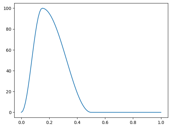
Activation Model (Synthetic)#
We use the Blanco time-varying elastance function for a synthetic activation trace. We use a peak activation of 100 kPa to match typical ventricular pressures, with the time to peak at 150 ms and relaxation until 350 ms, and a total cycle length of 1 s.
def get_activation(t):
    return 100 * circulation.time_varying_elastance.blanco_ventricle(
        EA=1.0,
        EB=0.0,
        tC=0.0,
        TC=0.15,
        TR=0.35,
        RR=1.0,
    )(t)
Let us plot the resulting activation trace
if comm.rank == 0:
    fig, ax = plt.subplots()
    t = np.linspace(0, 1, 100)
    ax.plot(t, get_activation(t))
    fig.savefig(outdir / "activation.png")
def setup_problem(geometry, f0, s0, material_params):
    material = pulse.HolzapfelOgden(f0=f0, s0=s0, **material_params)
    Ta = pulse.Variable(
        dolfinx.fem.Constant(geometry.mesh, dolfinx.default_scalar_type(0.0)),
        "kPa",
    )
    active_model = pulse.ActiveStress(f0, activation=Ta)
    comp_model = pulse.compressibility.Compressible2()

    model = pulse.CardiacModel(
        material=material,
        active=active_model,
        compressibility=comp_model,
    )

    alpha_epi = pulse.Variable(
        dolfinx.fem.Constant(geometry.mesh, dolfinx.default_scalar_type(1e5)),
        "Pa / m",
    )
    robin_epi = pulse.RobinBC(value=alpha_epi, marker=geometry.markers["EPI"][0])

    alpha_base = pulse.Variable(
        dolfinx.fem.Constant(geometry.mesh, dolfinx.default_scalar_type(1e6)),
        "Pa / m",
    )
    robin_base = pulse.RobinBC(value=alpha_base, marker=geometry.markers["BASE"][0])

    robin = [robin_epi, robin_base]

    # Dirichlet BC: Sliding Base (ux=0)
    def dirichlet_bc(V: dolfinx.fem.FunctionSpace):
        facets = geometry.facet_tags.find(geometry.markers["BASE"][0])
        dofs = dolfinx.fem.locate_dofs_topological(V.sub(0), 2, facets)
        return [dolfinx.fem.dirichletbc(0.0, dofs, V.sub(0))]

    return model, robin, dirichlet_bc, Ta
material_params = pulse.HolzapfelOgden.transversely_isotropic_parameters()
model, robin, dirichlet_bc, Ta = setup_problem(
    geometry=geometry,
    f0=geo.f0,
    s0=geo.s0,
    material_params=material_params,
)
Prestressing (Inverse Elasticity)#
We use the target ED pressures from the 0D circulation model to prestress the mesh.
p_LV_ED = mmHg_to_kPa(history["p_LV"][-1])
p_RV_ED = mmHg_to_kPa(history["p_RV"][-1])
logger.info(
    f"Target ED Pressures from 0D: p_LV={p_LV_ED:.2f} kPa, p_RV={p_RV_ED:.2f} kPa",
)
[06/30/26 21:16:51] INFO INFO:pulse:Target ED Pressures from 0D: p_LV=1.62 kPa, p_RV=0.54 kPa 2268742762.py:1
Since we want to apply pressures on both ventricles, we create two Neumann BCs.
pressure_lv = pulse.Variable(dolfinx.fem.Constant(geometry.mesh, 0.0), "kPa")
pressure_rv = pulse.Variable(dolfinx.fem.Constant(geometry.mesh, 0.0), "kPa")
neumann_lv = pulse.NeumannBC(traction=pressure_lv, marker=geometry.markers["LV"][0])
neumann_rv = pulse.NeumannBC(traction=pressure_rv, marker=geometry.markers["RV"][0])
bcs_prestress = pulse.BoundaryConditions(
    robin=robin,
    dirichlet=(dirichlet_bc,),
    neumann=(neumann_lv, neumann_rv),
)
We store the prestressed displacement in a file to avoid recomputing it.
prestress_fname = outdir / "prestress_biv_inverse.bp"
if not prestress_fname.exists():
    logger.info(
        f"Start prestressing... Targets: p_LV={p_LV_ED:.2f} kPa, p_RV={p_RV_ED:.2f} kPa",
    )
    prestress_problem = pulse.unloading.PrestressProblem(
        geometry=geometry,
        model=model,
        bcs=bcs_prestress,
        parameters={"u_space": "P_2", "mesh_unit": mesh_unit},
        targets=[
            pulse.unloading.TargetPressure(
                traction=pressure_lv, target=p_LV_ED, name="LV",
            ),
            pulse.unloading.TargetPressure(
                traction=pressure_rv, target=p_RV_ED, name="RV",
            ),
        ],
        ramp_steps=20,
    )

    u_pre = prestress_problem.unload()
    io4dolfinx.write_function_on_input_mesh(
        prestress_fname, u_pre, time=0.0, name="u_pre",
    )
    with dolfinx.io.VTXWriter(
        comm,
        outdir / "prestress_biv_backward.bp",
        [u_pre],
        engine="BP4",
    ) as vtx:
        vtx.write(0.0)
INFO INFO:pulse:Start prestressing... Targets: p_LV=1.62 kPa, p_RV=0.54 kPa 1909972065.py:3
[06/30/26 21:16:57] INFO INFO:pulse.unloading:Ramping LV traction to 0.0000 unloading.py:490
INFO INFO:pulse.unloading:Ramping RV traction to 0.0000 unloading.py:490
[06/30/26 21:16:58] INFO INFO:pulse.unloading:Ramping LV traction to 0.0850 unloading.py:490
INFO INFO:pulse.unloading:Ramping RV traction to 0.0286 unloading.py:490
[06/30/26 21:17:00] INFO INFO:pulse.unloading:Ramping LV traction to 0.1700 unloading.py:490
INFO INFO:pulse.unloading:Ramping RV traction to 0.0571 unloading.py:490
[06/30/26 21:17:03] INFO INFO:pulse.unloading:Ramping LV traction to 0.2550 unloading.py:490
INFO INFO:pulse.unloading:Ramping RV traction to 0.0857 unloading.py:490
[06/30/26 21:17:05] INFO INFO:pulse.unloading:Ramping LV traction to 0.3400 unloading.py:490
INFO INFO:pulse.unloading:Ramping RV traction to 0.1143 unloading.py:490
[06/30/26 21:17:07] INFO INFO:pulse.unloading:Ramping LV traction to 0.4250 unloading.py:490
INFO INFO:pulse.unloading:Ramping RV traction to 0.1428 unloading.py:490
[06/30/26 21:17:10] INFO INFO:pulse.unloading:Ramping LV traction to 0.5101 unloading.py:490
INFO INFO:pulse.unloading:Ramping RV traction to 0.1714 unloading.py:490
[06/30/26 21:17:12] INFO INFO:pulse.unloading:Ramping LV traction to 0.5951 unloading.py:490
INFO INFO:pulse.unloading:Ramping RV traction to 0.2000 unloading.py:490
[06/30/26 21:17:14] INFO INFO:pulse.unloading:Ramping LV traction to 0.6801 unloading.py:490
INFO INFO:pulse.unloading:Ramping RV traction to 0.2286 unloading.py:490
[06/30/26 21:17:17] INFO INFO:pulse.unloading:Ramping LV traction to 0.7651 unloading.py:490
INFO INFO:pulse.unloading:Ramping RV traction to 0.2571 unloading.py:490
[06/30/26 21:17:19] INFO INFO:pulse.unloading:Ramping LV traction to 0.8501 unloading.py:490
INFO INFO:pulse.unloading:Ramping RV traction to 0.2857 unloading.py:490
[06/30/26 21:17:21] INFO INFO:pulse.unloading:Ramping LV traction to 0.9351 unloading.py:490
INFO INFO:pulse.unloading:Ramping RV traction to 0.3143 unloading.py:490
[06/30/26 21:17:24] INFO INFO:pulse.unloading:Ramping LV traction to 1.0201 unloading.py:490
INFO INFO:pulse.unloading:Ramping RV traction to 0.3428 unloading.py:490
[06/30/26 21:17:25] INFO INFO:pulse.unloading:Ramping LV traction to 1.1051 unloading.py:490
INFO INFO:pulse.unloading:Ramping RV traction to 0.3714 unloading.py:490
[06/30/26 21:17:27] INFO INFO:pulse.unloading:Ramping LV traction to 1.1901 unloading.py:490
INFO INFO:pulse.unloading:Ramping RV traction to 0.4000 unloading.py:490
[06/30/26 21:17:29] INFO INFO:pulse.unloading:Ramping LV traction to 1.2751 unloading.py:490
INFO INFO:pulse.unloading:Ramping RV traction to 0.4285 unloading.py:490
[06/30/26 21:17:31] INFO INFO:pulse.unloading:Ramping LV traction to 1.3602 unloading.py:490
INFO INFO:pulse.unloading:Ramping RV traction to 0.4571 unloading.py:490
[06/30/26 21:17:33] INFO INFO:pulse.unloading:Ramping LV traction to 1.4452 unloading.py:490
INFO INFO:pulse.unloading:Ramping RV traction to 0.4857 unloading.py:490
[06/30/26 21:17:34] INFO INFO:pulse.unloading:Ramping LV traction to 1.5302 unloading.py:490
INFO INFO:pulse.unloading:Ramping RV traction to 0.5142 unloading.py:490
[06/30/26 21:17:36] INFO INFO:pulse.unloading:Ramping LV traction to 1.6152 unloading.py:490
INFO INFO:pulse.unloading:Ramping RV traction to 0.5428 unloading.py:490
Forward Problem Setup#
V = dolfinx.fem.functionspace(geometry.mesh, ("Lagrange", 2, (3,)))
u_pre = dolfinx.fem.Function(V)
io4dolfinx.read_function(prestress_fname, u_pre, time=0.0, name="u_pre")
We use the prestressed displacement to deform the mesh to the reference configuration.
logger.info("Deforming mesh to Reference Configuration...")
geometry.deform(u_pre)
[06/30/26 21:17:38] INFO INFO:pulse:Deforming mesh to Reference Configuration... 255936268.py:1
We now map the fiber fields to the reference configuration.
logger.info("Mapping fibers to Reference Configuration...")
f0_quad = pulse.utils.map_vector_field(
    f=geo.f0, u=u_pre, normalize=True, name="f0_unloaded",
)
s0_quad = pulse.utils.map_vector_field(
    f=geo.s0, u=u_pre, normalize=True, name="s0_unloaded",
)
f0_map = pulse.utils.map_vector_field(
    geo.additional_data["f0_DG_1"],
    u=u_pre,
    normalize=True,
    name="f0",
)
INFO INFO:pulse:Mapping fibers to Reference Configuration... 372092683.py:1
Calculate unloaded volumes
lvv_unloaded = comm.allreduce(geometry.volume("LV"), op=MPI.SUM)
rvv_unloaded = comm.allreduce(geometry.volume("RV"), op=MPI.SUM)
logger.info(
    f"Unloaded volumes: LV={lvv_unloaded * volume2ml:.2f} mL, RV={rvv_unloaded * volume2ml:.2f} mL",
)
model, robin, dirichlet_bc, Ta = setup_problem(
    geometry=geometry,
    f0=f0_quad,
    s0=s0_quad,
    material_params=material_params,
)
INFO INFO:pulse:Unloaded volumes: LV=75.23 mL, RV=59.40 mL 1709951115.py:3
Since we will be applying volume constraints, we define cavities for both ventricles.
lv_volume = dolfinx.fem.Constant(
    geometry.mesh, dolfinx.default_scalar_type(lvv_unloaded),
)
rv_volume = dolfinx.fem.Constant(
    geometry.mesh, dolfinx.default_scalar_type(rvv_unloaded),
)
cavities = [
    pulse.problem.Cavity(marker="LV", volume=lv_volume),
    pulse.problem.Cavity(marker="RV", volume=rv_volume),
]
bcs_forward = pulse.BoundaryConditions(robin=robin, dirichlet=(dirichlet_bc,))
problem = pulse.problem.StaticProblem(
    model=model,
    geometry=geometry,
    bcs=bcs_forward,
    cavities=cavities,
    parameters={"mesh_unit": mesh_unit, "u_space": "P_2"},
)
We set up functions to compute fiber stress and fiber strain during the simulation for post-processing.
W = dolfinx.fem.functionspace(geometry.mesh, ("DG", 1))
I = ufl.Identity(3)
F = ufl.variable(ufl.grad(problem.u) + I)
C = F.T * F
E = 0.5 * (C - I)
Mapped fiber direction in current config used for the Cauchy stress calculation
Material for stress calc
material_dg = pulse.HolzapfelOgden(f0=f0_map, s0=f0_map, **material_params)
T = material_dg.sigma(F)
We define functions to store fiber stress and strain, as well as their expressions.
fiber_stress = dolfinx.fem.Function(W, name="fiber_stress")
fiber_stress_expr = dolfinx.fem.Expression(
    ufl.inner(T * f_map, f_map),
    W.element.interpolation_points,
)
fiber_strain = dolfinx.fem.Function(W, name="fiber_strain")
fiber_strain_expr = dolfinx.fem.Expression(
    ufl.inner(E * f0_map, f0_map),
    W.element.interpolation_points,
)
VTX Writers for visualization in ParaView
vtx = dolfinx.io.VTXWriter(
    geometry.mesh.comm,
    outdir / "displacement.bp",
    [problem.u],
    engine="BP4",
)
vtx_stress = dolfinx.io.VTXWriter(
    geometry.mesh.comm,
    outdir / "stress_strain.bp",
    [fiber_stress, fiber_strain],
    engine="BP4",
)
8. Inflation (Reference -> End-Diastole)#
We now ramp the volumes from the unloaded state back to the target ED volumes. This establishes the correct initial condition (stress/strain) for the time-dependent loop.
logger.info("Inflating to End-Diastolic Target...")
ramp_steps = 10
for i in range(ramp_steps):
    factor = (i + 1) / ramp_steps

    # Interpolate volume
    current_lvv = lvv_unloaded + factor * (lvv_target - lvv_unloaded)
    current_rvv = rvv_unloaded + factor * (rvv_target - rvv_unloaded)

    lv_volume.value = current_lvv
    rv_volume.value = current_rvv

    problem.solve()

    # Log pressures to ensure we are reaching target
    plv = problem.cavity_pressures[0].x.array[0] * 1e-3
    prv = problem.cavity_pressures[1].x.array[0] * 1e-3
    if comm.rank == 0:
        logger.info(
            f"Inflation Step {i + 1}/{ramp_steps}: pLV={plv:.2f} kPa, pRV={prv:.2f} kPa",
        )
[06/30/26 21:17:59] INFO INFO:pulse:Inflating to End-Diastolic Target... 3195246893.py:1
[06/30/26 21:18:05] INFO INFO:pulse:Inflation Step 1/10: pLV=0.09 kPa, pRV=0.04 kPa 3195246893.py:19
[06/30/26 21:18:12] INFO INFO:pulse:Inflation Step 2/10: pLV=0.19 kPa, pRV=0.09 kPa 3195246893.py:19
[06/30/26 21:18:18] INFO INFO:pulse:Inflation Step 3/10: pLV=0.28 kPa, pRV=0.13 kPa 3195246893.py:19
[06/30/26 21:18:25] INFO INFO:pulse:Inflation Step 4/10: pLV=0.39 kPa, pRV=0.18 kPa 3195246893.py:19
[06/30/26 21:18:31] INFO INFO:pulse:Inflation Step 5/10: pLV=0.50 kPa, pRV=0.23 kPa 3195246893.py:19
[06/30/26 21:18:38] INFO INFO:pulse:Inflation Step 6/10: pLV=0.63 kPa, pRV=0.28 kPa 3195246893.py:19
[06/30/26 21:18:44] INFO INFO:pulse:Inflation Step 7/10: pLV=0.77 kPa, pRV=0.33 kPa 3195246893.py:19
[06/30/26 21:18:51] INFO INFO:pulse:Inflation Step 8/10: pLV=0.94 kPa, pRV=0.38 kPa 3195246893.py:19
[06/30/26 21:18:57] INFO INFO:pulse:Inflation Step 9/10: pLV=1.14 kPa, pRV=0.44 kPa 3195246893.py:19
[06/30/26 21:19:04] INFO INFO:pulse:Inflation Step 10/10: pLV=1.37 kPa, pRV=0.50 kPa 3195246893.py:19
vtx.write(0.0)
vtx_stress.write(0.0)
Store old values for time-stepping and handling if solver fails
problem.old_Ta = Ta.value.value.copy()  # type: ignore
problem.old_lv_volume = lv_volume.value.copy()  # type: ignore
problem.old_rv_volume = rv_volume.value.copy()  # type: ignore
10. Multiscale Coupling Loop#
def p_BiV_func(V_LV, V_RV, t):
    logger.info(f"Coupling Time {t:.4f}: Target V_LV={V_LV:.2f}, V_RV={V_RV:.2f}")
    value = get_activation(t)
    old_Ta = problem.old_Ta
    dTa = value - old_Ta

    # We compute the new target volumes accounting for the errors from the initial 0D run
    new_value_LV = (V_LV - error_LV) * (1.0 / volume2ml)
    new_value_RV = (V_RV - error_RV) * (1.0 / volume2ml)

    old_lv_volume = problem.old_lv_volume
    old_rv_volume = problem.old_rv_volume

    dLV = new_value_LV - old_lv_volume
    dRV = new_value_RV - old_rv_volume

    converged = False
    num_failures = 0
    num_steps = 1
    tol = 1e-12

    old_lv_it = old_lv_volume.copy()
    old_rv_it = old_rv_volume.copy()
    old_Ta = Ta.value.value.copy()

    # Only attempt to solve if there is a change in any of the targets
    if abs(dLV) > tol or abs(dRV) > tol or abs(dTa) > tol:
        while not converged and num_failures < 20:
            for i in range(num_steps):
                lv_volume.value = (
                    old_lv_volume + (i + 1) * (new_value_LV - old_lv_it) / num_steps
                )
                rv_volume.value = (
                    old_rv_volume + (i + 1) * (new_value_RV - old_rv_it) / num_steps
                )
                Ta.assign(old_Ta + (i + 1) * dTa / num_steps)
                try:
                    problem.solve()
                except RuntimeError as e:
                    print(f"Error during solve: {e}")
                    # If the solve fails, we reset the volumes and Ta to the old values
                    lv_volume.value = old_lv_volume.copy()
                    rv_volume.value = old_rv_volume.copy()
                    Ta.assign(old_Ta)
                    problem.reset()
                    num_failures += 1
                    num_steps *= 2
                    converged = False
                else:
                    converged = True
                    old_lv_it = lv_volume.value.copy()
                    old_rv_it = rv_volume.value.copy()
                    old_Ta = Ta.value.value.copy()

            if not converged:
                print(
                    f"Failed to converge after {num_failures} attempts. "
                    f"LV volume: {new_value_LV}, RV volume: {new_value_RV}, Ta: {value}",
                )
                raise RuntimeError("Failed to converge on pressure calculation.")

    problem.old_Ta = Ta.value.value.copy()  # type: ignore
    problem.old_lv_volume = lv_volume.value.copy()  # type: ignore
    problem.old_rv_volume = rv_volume.value.copy()  # type: ignore

    lv_p_kPa = problem.cavity_pressures[0].x.array[0] * 1e-3
    rv_p_kPa = problem.cavity_pressures[1].x.array[0] * 1e-3

    return circulation.units.kPa_to_mmHg(lv_p_kPa), circulation.units.kPa_to_mmHg(
        rv_p_kPa,
    )
Write checkpoint of mesh meshtags, and functions for postprocessing
filename = outdir / Path("function_checkpoint.bp")
shutil.rmtree(filename, ignore_errors=True)
io4dolfinx.write_mesh(filename, geometry.mesh)
io4dolfinx.write_meshtags(
    filename, mesh=geometry.mesh, meshtags=geometry.facet_tags, meshtag_name="ffun",
)
output_file = outdir / "output.json"
Ta_history: list[float] = []
def callback(model, i: int, t: float, save=True):
    fiber_stress.interpolate(fiber_stress_expr)
    fiber_strain.interpolate(fiber_strain_expr)
    Ta_history.append(get_activation(t))

    if save:
        vtx.write(t)
        vtx_stress.write(t)
        io4dolfinx.write_function(filename, u=problem.u, name="displacement", time=t)
        io4dolfinx.write_function(filename, u=fiber_stress, name="fiber_stress", time=t)
        io4dolfinx.write_function(filename, u=fiber_strain, name="fiber_strain", time=t)
        out = {k: v[: i + 1] for k, v in model.history.items()}
        out["Ta"] = Ta_history
        V_LV = model.history["V_LV"][: i + 1] - error_LV
        V_RV = model.history["V_RV"][: i + 1] - error_RV
        out["V_LV"] = V_LV
        out["V_RV"] = V_RV
        if comm.rank == 0:
            output_file.write_text(json.dumps(out, indent=4, default=custom_json))

            # Plot PV loops and other quantities incrementally
            fig = plt.figure(layout="constrained", figsize=(12, 8))
            gs = GridSpec(3, 4, figure=fig)
            ax1 = fig.add_subplot(gs[:, 0])
            ax2 = fig.add_subplot(gs[:, 1])
            ax3 = fig.add_subplot(gs[0, 2])
            ax4 = fig.add_subplot(gs[1, 2])
            ax5 = fig.add_subplot(gs[0, 3])
            ax6 = fig.add_subplot(gs[1, 3])
            ax7 = fig.add_subplot(gs[2, 2:])

            p_LV = model.history["p_LV"][: i + 1]
            p_RV = model.history["p_RV"][: i + 1]

            ax1.plot(V_LV, p_LV)
            ax1.set_xlabel("LVV [mL]")
            ax1.set_ylabel("LVP [mmHg]")

            ax2.plot(V_RV, p_RV)
            ax2.set_xlabel("RVV [mL]")
            ax2.set_ylabel("RVP [mmHg]")

            ax3.plot(model.history["time"][: i + 1], p_LV)
            ax3.set_ylabel("LVP [mmHg]")
            ax4.plot(model.history["time"][: i + 1], V_LV)
            ax4.set_ylabel("LVV [mL]")

            ax5.plot(model.history["time"][: i + 1], p_RV)
            ax5.set_ylabel("RVP [mmHg]")
            ax6.plot(model.history["time"][: i + 1], V_RV)
            ax6.set_ylabel("RVV [mL]")

            ax7.plot(model.history["time"][: i + 1], Ta_history[: i + 1])
            ax7.set_ylabel("Ta [kPa]")

            for axi in [ax3, ax4, ax5, ax6, ax7]:
                axi.set_xlabel("Time [s]")

            fig.savefig(outdir / "pv_loop_incremental.png")
            plt.close(fig)
Initialize Circulation Model with Target (ED) Volumes
circulation_model = circulation.regazzoni2020.Regazzoni2020(
    add_units=False,
    callback=callback,
    p_BiV=p_BiV_func,
    verbose=True,
    comm=comm,
    outdir=outdir,
)
                    INFO     INFO:circulation.base:                                                                                                                                          base.py:134
                                                    Circulation model parameters (Regazzoni2020)
                             ┏━━━━━━━━━━━━━━━━━━━━━━━━━━━━━━━━━━━━━━━┳━━━━━━━━━━━━━━━━━━━━━━━━━━━━━━━━━━━━━━━━━━━━━━━━━┓
                             ┃ Parameter                             ┃ Value                                           ┃
                             ┡━━━━━━━━━━━━━━━━━━━━━━━━━━━━━━━━━━━━━━━╇━━━━━━━━━━━━━━━━━━━━━━━━━━━━━━━━━━━━━━━━━━━━━━━━━┩
                             │ HR                                    │ 1.25 hertz                                      │
                             │ chambers.LA.EA                        │ 0.07 millimeter_Hg / milliliter                 │
                             │ chambers.LA.EB                        │ 0.18 millimeter_Hg / milliliter                 │
                             │ chambers.LA.TC                        │ 0.17 second                                     │
                             │ chambers.LA.TR                        │ 0.17 second                                     │
                             │ chambers.LA.tC                        │ 0.9 second                                      │
                             │ chambers.LA.V0                        │ 4.0 milliliter                                  │
                             │ chambers.LV.EA                        │ 4.482 millimeter_Hg / milliliter                │
                             │ chambers.LV.EB                        │ 0.17 millimeter_Hg / milliliter                 │
                             │ chambers.LV.TC                        │ 0.25 second                                     │
                             │ chambers.LV.TR                        │ 0.4 second                                      │
                             │ chambers.LV.tC                        │ 0.1 second                                      │
                             │ chambers.LV.V0                        │ 42.0 milliliter                                 │
                             │ chambers.RA.EA                        │ 0.06 millimeter_Hg / milliliter                 │
                             │ chambers.RA.EB                        │ 0.07 millimeter_Hg / milliliter                 │
                             │ chambers.RA.TC                        │ 0.17 second                                     │
                             │ chambers.RA.TR                        │ 0.17 second                                     │
                             │ chambers.RA.tC                        │ 0.9 second                                      │
                             │ chambers.RA.V0                        │ 4.0 milliliter                                  │
                             │ chambers.RV.EA                        │ 0.2 millimeter_Hg / milliliter                  │
                             │ chambers.RV.EB                        │ 0.029 millimeter_Hg / milliliter                │
                             │ chambers.RV.TC                        │ 0.25 second                                     │
                             │ chambers.RV.TR                        │ 0.4 second                                      │
                             │ chambers.RV.tC                        │ 0.1 second                                      │
                             │ chambers.RV.V0                        │ 16.0 milliliter                                 │
                             │ valves.MV.Rmin                        │ 0.0075 millimeter_Hg * second / milliliter      │
                             │ valves.MV.Rmax                        │ 75006.2 millimeter_Hg * second / milliliter     │
                             │ valves.AV.Rmin                        │ 0.0075 millimeter_Hg * second / milliliter      │
                             │ valves.AV.Rmax                        │ 75006.2 millimeter_Hg * second / milliliter     │
                             │ valves.TV.Rmin                        │ 0.0075 millimeter_Hg * second / milliliter      │
                             │ valves.TV.Rmax                        │ 75006.2 millimeter_Hg * second / milliliter     │
                             │ valves.PV.Rmin                        │ 0.0075 millimeter_Hg * second / milliliter      │
                             │ valves.PV.Rmax                        │ 75006.2 millimeter_Hg * second / milliliter     │
                             │ circulation.SYS.R_AR                  │ 0.733 millimeter_Hg * second / milliliter       │
                             │ circulation.SYS.C_AR                  │ 1.372 milliliter / millimeter_Hg                │
                             │ circulation.SYS.R_VEN                 │ 0.32 millimeter_Hg * second / milliliter        │
                             │ circulation.SYS.C_VEN                 │ 11.363 milliliter / millimeter_Hg               │
                             │ circulation.SYS.L_AR                  │ 0.005 millimeter_Hg * second ** 2 / milliliter  │
                             │ circulation.SYS.L_VEN                 │ 0.0005 millimeter_Hg * second ** 2 / milliliter │
                             │ circulation.PUL.R_AR                  │ 0.046 millimeter_Hg * second / milliliter       │
                             │ circulation.PUL.C_AR                  │ 20.0 milliliter / millimeter_Hg                 │
                             │ circulation.PUL.R_VEN                 │ 0.0015 millimeter_Hg * second / milliliter      │
                             │ circulation.PUL.C_VEN                 │ 16.0 milliliter / millimeter_Hg                 │
                             │ circulation.PUL.L_AR                  │ 0.0005 millimeter_Hg * second ** 2 / milliliter │
                             │ circulation.PUL.L_VEN                 │ 0.0005 millimeter_Hg * second ** 2 / milliliter │
                             │ circulation.external.start_withdrawal │ 0.0 second                                      │
                             │ circulation.external.end_withdrawal   │ 0.0 second                                      │
                             │ circulation.external.start_infusion   │ 0.0 second                                      │
                             │ circulation.external.end_infusion     │ 0.0 second                                      │
                             │ circulation.external.flow_withdrawal  │ 0.0 milliliter / second                         │
                             │ circulation.external.flow_infusion    │ 0.0 milliliter / second                         │
                             └───────────────────────────────────────┴─────────────────────────────────────────────────┘
                    INFO     INFO:circulation.base:                                                                                                                                          base.py:141
                                  Circulation model initial states
                                           (Regazzoni2020)
                             ┏━━━━━━━━━━━┳━━━━━━━━━━━━━━━━━━━━━━━━━━━━━┓
                             ┃ State     ┃ Value                       ┃
                             ┡━━━━━━━━━━━╇━━━━━━━━━━━━━━━━━━━━━━━━━━━━━┩
                             │ V_LA      │ 87.183 milliliter           │
                             │ V_LV      │ 118.52 milliliter           │
                             │ V_RA      │ 86.833 milliliter           │
                             │ V_RV      │ 166.177 milliliter          │
                             │ p_AR_SYS  │ 87.675 millimeter_Hg        │
                             │ p_VEN_SYS │ 35.898 millimeter_Hg        │
                             │ p_AR_PUL  │ 19.545 millimeter_Hg        │
                             │ p_VEN_PUL │ 15.004 millimeter_Hg        │
                             │ Q_AR_SYS  │ 71.104 milliliter / second  │
                             │ Q_VEN_SYS │ 94.039 milliliter / second  │
                             │ Q_AR_PUL  │ 94.084 milliliter / second  │
                             │ Q_VEN_PUL │ 473.279 milliliter / second │
                             └───────────┴─────────────────────────────┘
logger.info("Starting coupled simulation...")
num_beats = 8
dt = 0.001
end_time = 2 * dt if os.getenv("CI") else None
circulation_model.solve(
    num_beats=num_beats, initial_state=circ_state, dt=dt, T=end_time,
)
logger.info("Simulation complete.")
INFO INFO:pulse:Coupling Time 0.0000: Target V_LV=113.50, V_RV=156.57 75630478.py:2
INFO INFO:pulse:Coupling Time 0.0000: Target V_LV=113.50, V_RV=156.57 75630478.py:2
[06/30/26 21:19:05] INFO     INFO:circulation.base:                                                                                                                                          base.py:512
                                                                                        Volumes
                             ┏━━━━━━━━┳━━━━━━━━━┳━━━━━━━━┳━━━━━━━━━┳━━━━━━━━━━┳━━━━━━━━━━━┳━━━━━━━━━━┳━━━━━━━━━━━┳━━━━━━━━━┳━━━━━━━━━┳━━━━━━━━━┳━━━━━━━━━━┓
                             ┃ V_LA   ┃ V_LV    ┃ V_RA   ┃ V_RV    ┃ V_AR_SYS ┃ V_VEN_SYS ┃ V_AR_PUL ┃ V_VEN_PUL ┃ Heart   ┃ SYS     ┃ PUL     ┃ Total    ┃
                             ┡━━━━━━━━╇━━━━━━━━━╇━━━━━━━━╇━━━━━━━━━╇━━━━━━━━━━╇━━━━━━━━━━━╇━━━━━━━━━━╇━━━━━━━━━━━╇━━━━━━━━━╇━━━━━━━━━╇━━━━━━━━━╇━━━━━━━━━━┩
                             │ 81.566 │ 113.990 │ 81.408 │ 156.796 │ 112.396  │ 383.039   │ 364.652  │ 223.347   │ 433.761 │ 495.436 │ 587.999 │ 1517.195 │
                             └────────┴─────────┴────────┴─────────┴──────────┴───────────┴──────────┴───────────┴─────────┴─────────┴─────────┴──────────┘

                                                                 Pressures
                             ┏━━━━━━━━┳━━━━━━━━┳━━━━━━━┳━━━━━━━┳━━━━━━━━━━┳━━━━━━━━━━━┳━━━━━━━━━━┳━━━━━━━━━━━┓
                             ┃ p_LA   ┃ p_LV   ┃ p_RA  ┃ p_RV  ┃ p_AR_SYS ┃ p_VEN_SYS ┃ p_AR_PUL ┃ p_VEN_PUL ┃
                             ┡━━━━━━━━╇━━━━━━━━╇━━━━━━━╇━━━━━━━╇━━━━━━━━━━╇━━━━━━━━━━━╇━━━━━━━━━━╇━━━━━━━━━━━┩
                             │ 13.970 │ 10.311 │ 5.428 │ 3.741 │ 81.921   │ 33.709    │ 18.233   │ 13.959    │
                             └────────┴────────┴───────┴───────┴──────────┴───────────┴──────────┴───────────┘

                                                                     Flows
                             ┏━━━━━━━━━┳━━━━━━━━┳━━━━━━━━━┳━━━━━━━━┳━━━━━━━━━━┳━━━━━━━━━━━┳━━━━━━━━━━┳━━━━━━━━━━━┓
                             ┃ Q_MV    ┃ Q_AV   ┃ Q_TV    ┃ Q_PV   ┃ Q_AR_SYS ┃ Q_VEN_SYS ┃ Q_AR_PUL ┃ Q_VEN_PUL ┃
                             ┡━━━━━━━━━╇━━━━━━━━╇━━━━━━━━━╇━━━━━━━━╇━━━━━━━━━━╇━━━━━━━━━━━╇━━━━━━━━━━╇━━━━━━━━━━━┩
                             │ 485.734 │ -0.001 │ 222.804 │ -0.000 │ 66.208   │ 88.378    │ 88.659   │ 437.103   │
                             └─────────┴────────┴─────────┴────────┴──────────┴───────────┴──────────┴───────────┘
INFO INFO:pulse:Coupling Time 0.0010: Target V_LV=113.99, V_RV=156.80 75630478.py:2
[06/30/26 21:19:09] INFO     INFO:circulation.base:                                                                                                                                          base.py:512
                                                                                        Volumes
                             ┏━━━━━━━━┳━━━━━━━━━┳━━━━━━━━┳━━━━━━━━━┳━━━━━━━━━━┳━━━━━━━━━━━┳━━━━━━━━━━┳━━━━━━━━━━━┳━━━━━━━━━┳━━━━━━━━━┳━━━━━━━━━┳━━━━━━━━━━┓
                             ┃ V_LA   ┃ V_LV    ┃ V_RA   ┃ V_RV    ┃ V_AR_SYS ┃ V_VEN_SYS ┃ V_AR_PUL ┃ V_VEN_PUL ┃ Heart   ┃ SYS     ┃ PUL     ┃ Total    ┃
                             ┡━━━━━━━━╇━━━━━━━━━╇━━━━━━━━╇━━━━━━━━━╇━━━━━━━━━━╇━━━━━━━━━━━╇━━━━━━━━━━╇━━━━━━━━━━━╇━━━━━━━━━╇━━━━━━━━━╇━━━━━━━━━╇━━━━━━━━━━┩
                             │ 81.559 │ 114.435 │ 81.284 │ 157.008 │ 112.330  │ 383.017   │ 364.563  │ 222.998   │ 434.286 │ 495.347 │ 587.562 │ 1517.195 │
                             └────────┴─────────┴────────┴─────────┴──────────┴───────────┴──────────┴───────────┴─────────┴─────────┴─────────┴──────────┘

                                                                 Pressures
                             ┏━━━━━━━━┳━━━━━━━━┳━━━━━━━┳━━━━━━━┳━━━━━━━━━━┳━━━━━━━━━━━┳━━━━━━━━━━┳━━━━━━━━━━━┓
                             ┃ p_LA   ┃ p_LV   ┃ p_RA  ┃ p_RV  ┃ p_AR_SYS ┃ p_VEN_SYS ┃ p_AR_PUL ┃ p_VEN_PUL ┃
                             ┡━━━━━━━━╇━━━━━━━━╇━━━━━━━╇━━━━━━━╇━━━━━━━━━━╇━━━━━━━━━━━╇━━━━━━━━━━╇━━━━━━━━━━━┩
                             │ 13.962 │ 10.610 │ 5.419 │ 3.814 │ 81.873   │ 33.707    │ 18.228   │ 13.937    │
                             └────────┴────────┴───────┴───────┴──────────┴───────────┴──────────┴───────────┘

                                                                     Flows
                             ┏━━━━━━━━━┳━━━━━━━━┳━━━━━━━━━┳━━━━━━━━┳━━━━━━━━━━┳━━━━━━━━━━━┳━━━━━━━━━━┳━━━━━━━━━━━┓
                             ┃ Q_MV    ┃ Q_AV   ┃ Q_TV    ┃ Q_PV   ┃ Q_AR_SYS ┃ Q_VEN_SYS ┃ Q_AR_PUL ┃ Q_VEN_PUL ┃
                             ┡━━━━━━━━━╇━━━━━━━━╇━━━━━━━━━╇━━━━━━━━╇━━━━━━━━━━╇━━━━━━━━━━━╇━━━━━━━━━━╇━━━━━━━━━━━┩
                             │ 444.767 │ -0.001 │ 211.745 │ -0.000 │ 66.144   │ 88.398    │ 89.049   │ 435.786   │
                             └─────────┴────────┴─────────┴────────┴──────────┴───────────┴──────────┴───────────┘
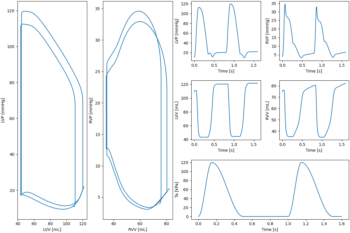
Fig. 4 Pressure volume loops#