LV ellipsoid coupled to a 0D circulatory model and a 0D cell model#
This example demonstrates a multiscale cardiac simulation coupling three distinct models:
3D Mechanics: An idealized Left Ventricle (LV) ellipsoid model solving the balance of linear momentum with active contraction.
0D Circulation: A lumped-parameter model of the closed-loop circulatory system [RSA+22].
0D Electrophysiology: A cellular model for human ventricular myocytes [TBOP+19] coupled with an excitation-contraction model [LPHS+17].
Coupling Strategy#
The coupling is achieved through a segregated approach:
Electrophysiology \(\rightarrow\) Mechanics: The 0D cell model (TorOrd-Land) is pre-solved to generate a time-dependent active tension transient \(T_a(t)\). This \(T_a(t)\) drives the active stress in the 3D mechanics model: \(\mathbf{S}_{active} = T_a(t) \mathbf{f}_0 \otimes \mathbf{f}_0\).
Circulation \(\leftrightarrow\) Mechanics: The 0D circulation model dictates the boundary conditions for the 3D mechanics model, and vice-versa. We use a volume-based coupling strategy:
The circulation model computes the new ventricular volume \(V_{n+1}\) at the next time step.
The 3D mechanics model solves a boundary value problem to find the cavity pressure \(P_{n+1}\) required to achieve this volume \(V_{n+1}\) (given the current activation \(T_a(t_{n+1})\)).
This pressure \(P_{n+1}\) is fed back to the circulation model.
Mathematical Models#
3D Mechanics#
Geometry: Idealized LV ellipsoid with fiber architecture.
Material: Transversely isotropic Holzapfel-Ogden model.
Active Stress: \(\mathbf{S}_{active} = T_a \mathbf{f}_0 \otimes \mathbf{f}_0\).
Boundary Conditions:
Epicardium & Base: Robin BCs (springs) to mimic pericardial constraint and prevent rigid body motion.
Endocardium: The pressure \(P\) is a Lagrange multiplier enforcing the volume constraint \(V(\mathbf{u}) = V_{target}\).
0D Circulation [Regazzoni et al. 2022]#
A closed-loop lumped-parameter network representing the systemic and pulmonary circulation. It includes 4 chambers (LA, LV, RA, RV) and systemic/pulmonary arteries and veins. In this example, we replace the 0D description of the LV with our 3D finite element model.
0D Cell Model [Tomek et al. 2019 + Land et al. 2017]#
TorOrd: Detailed human ventricular action potential model.
Land: Mechanical model describing cross-bridge dynamics and calcium binding to Troponin-C.
from pathlib import Path
from mpi4py import MPI
import dolfinx
import logging
import circulation
import os
import math
from functools import lru_cache
from dolfinx import log
from matplotlib.gridspec import GridSpec
import matplotlib.pyplot as plt
import numpy as np
import gotranx
import io4dolfinx
import pulse
import cardiac_geometries
import cardiac_geometries.geometry
Next we set up the logging and the MPI communicator
circulation.log.setup_logging(logging.INFO)
logging.getLogger("scifem").setLevel(logging.WARNING)
logger = logging.getLogger("pulse")
comm = MPI.COMM_WORLD
1. Geometry Generation#
We create the idealized LV geometry with appropriate fibers using cardiac_geometries.
geodir = Path("lv_ellipsoid-time-dependent")
if not geodir.exists():
    comm.barrier()
    cardiac_geometries.mesh.lv_ellipsoid(
        outdir=geodir,
        create_fibers=True,
        fiber_space="Quadrature_6",
        r_short_endo=0.025,
        r_short_epi=0.035,
        r_long_endo=0.09,
        r_long_epi=0.097,
        psize_ref=0.03,
        mu_apex_endo=-math.pi,
        mu_base_endo=-math.acos(5 / 17),
        mu_apex_epi=-math.pi,
        mu_base_epi=-math.acos(5 / 20),
        comm=comm,
        fiber_angle_epi=-60,
        fiber_angle_endo=60,
    )
Info    : Reading 'lv_ellipsoid-time-dependent/lv_ellipsoid.msh'...
Info    : 54 entities
Info    : 191 nodes
Info    : 990 elements
Info    : Done reading 'lv_ellipsoid-time-dependent/lv_ellipsoid.msh'
If the folder already exist, then we just load the geometry
geo = cardiac_geometries.geometry.Geometry.from_folder(
    comm=comm,
    folder=geodir,
)
[06/30/26 21:22:04] INFO INFO:cardiac_geometries.geometry:Reading geometry from lv_ellipsoid-time-dependent geometry.py:518
Next we transform the geometry to a HeartGeometry object
geometry = pulse.HeartGeometry.from_cardiac_geometries(
    geo, metadata={"quadrature_degree": 6},
)
2. Constitutive Model#
We use the standard Holzapfel-Ogden model for passive material properties and an Active Stress model driven by a scalar parameter \(T_a\).
material_params = pulse.HolzapfelOgden.transversely_isotropic_parameters()
material = pulse.HolzapfelOgden(f0=geo.f0, s0=geo.s0, **material_params)  # type: ignore
We use an active stress approach with 30% transverse active stress (see pulse.active_stress.transversely_active_stress())
Ta = pulse.Variable(
    dolfinx.fem.Constant(geometry.mesh, dolfinx.default_scalar_type(0.0)), "kPa",
)
active_model = pulse.ActiveStress(geo.f0, activation=Ta)
a compressible material model
and assembles the CardiacModel
model = pulse.CardiacModel(
    material=material,
    active=active_model,
    compressibility=comp_model,
)
3. Boundary Conditions#
We apply Robin boundary conditions (springs) to the epicardium and base to represent the pericardium and tissue support.
Crucially, for the endocardium, we use a Cavity Volume Constraint. Instead of applying a known pressure (Neumann BC), we enforce the cavity volume to match a target value provided by the circulation model. The Lagrange multiplier associated with this constraint is the cavity pressure.
alpha_epi = pulse.Variable(
    dolfinx.fem.Constant(geometry.mesh, dolfinx.default_scalar_type(1e8)),
    "Pa / m",
)
robin_epi = pulse.RobinBC(value=alpha_epi, marker=geometry.markers["EPI"][0])
alpha_base = pulse.Variable(
    dolfinx.fem.Constant(geometry.mesh, dolfinx.default_scalar_type(1e5)),
    "Pa / m",
)
robin_base = pulse.RobinBC(value=alpha_base, marker=geometry.markers["BASE"][0])
For the pressure we use a Lagrange multiplier method to enforce a given volume. The resulting Lagrange multiplier will be the pressure in the cavity.
To do this we create a Cavity object with a given volume, and specify which marker to use for the boundary condition.
initial_volume = geo.mesh.comm.allreduce(geometry.volume("ENDO"), op=MPI.SUM)
Volume = dolfinx.fem.Constant(
    geometry.mesh, dolfinx.default_scalar_type(initial_volume),
)
cavity = pulse.problem.Cavity(marker="ENDO", volume=Volume)
We also specify the parameters for the problem and say that we want the base to move freely and that the units of the mesh is meters
parameters = {"base_bc": pulse.problem.BaseBC.free, "mesh_unit": "m"}
# Next we set up the problem.
outdir = Path("lv_ellipsoid_time_dependent_circulation_static")
bcs = pulse.BoundaryConditions(robin=(robin_epi, robin_base))
problem = pulse.problem.StaticProblem(
    model=model, geometry=geometry, bcs=bcs, cavities=[cavity], parameters=parameters,
)
outdir.mkdir(exist_ok=True)
Now we can solve the problem
# log.set_log_level(log.LogLevel.INFO)
problem.solve()
True
We also use the time step from the problem to set the time step for the 0D cell model
dt = 0.001
times = np.arange(0.0, 1.0, dt)
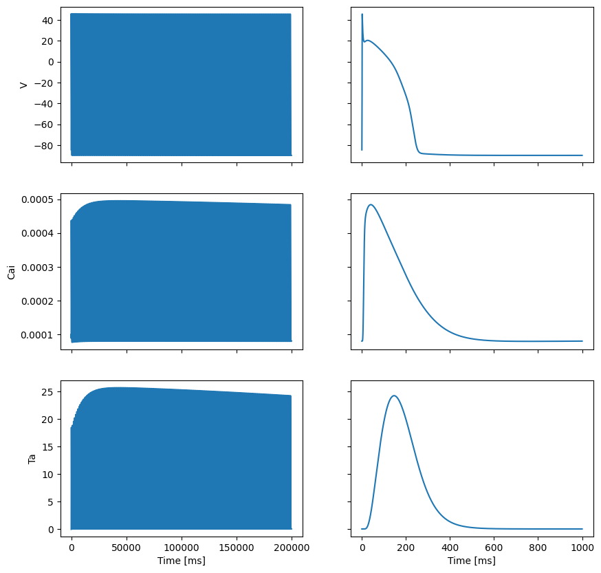
4. Electrophysiology (0D Cell Model)#
We pre-compute the active tension transient. We load the TorOrd-Land model using gotranx, solve it for 200 beats to reach a limit cycle (steady state), and save the final beat’s active tension trace.
if comm.rank == 0:
    ode = gotranx.load_ode("TorOrdLand.ode")
    ode = ode.remove_singularities()
    code = gotranx.cli.gotran2py.get_code(
        ode,
        scheme=[gotranx.schemes.Scheme.generalized_rush_larsen],
        shape=gotranx.codegen.base.Shape.single,
    )
    Path("TorOrdLand.py").write_text(code)
comm.barrier()
import TorOrdLand
2026-06-30 21:22:17 [info ] Load ode TorOrdLand.ode
2026-06-30 21:22:18 [info ] Num states 52
2026-06-30 21:22:18 [info ] Num parameters 140
TorOrdLand_model = TorOrdLand.__dict__
Ta_index = TorOrdLand_model["monitor_index"]("Ta")
y = TorOrdLand_model["init_state_values"]()
# Get initial parameter values
p = TorOrdLand_model["init_parameter_values"]()
import numba
fgr = numba.njit(TorOrdLand_model["generalized_rush_larsen"])
mon = numba.njit(TorOrdLand_model["monitor_values"])
V_index = TorOrdLand_model["state_index"]("v")
Ca_index = TorOrdLand_model["state_index"]("cai")
In the cell model the unit of time is in millisenconds, and we set the time step to 0.1 ms
# Time in milliseconds
dt_cell = 0.1
Now we solve the cell model for 200 beats and save the state at the end of the simulation
state_file = outdir / "state.npy"
if not state_file.is_file():

    @numba.jit(nopython=True)
    def solve_beat(times, states, dt, p, V_index, Ca_index, Vs, Cais, Tas):
        for i, ti in enumerate(times):
            states[:] = fgr(states, ti, dt, p)
            Vs[i] = states[V_index]
            Cais[i] = states[Ca_index]
            monitor = mon(ti, states, p)
            Tas[i] = monitor[Ta_index]

    # Time in milliseconds

    nbeats = 200
    T = 1000.00

    times = np.arange(0, T, dt_cell)
    all_times = np.arange(0, T * nbeats, dt_cell)
    Vs = np.zeros(len(times) * nbeats)
    Cais = np.zeros(len(times) * nbeats)
    Tas = np.zeros(len(times) * nbeats)
    logger.info(f"Starting to solve {nbeats} beats of the cell model")
    for beat in range(nbeats):
        logger.debug(f"Solving beat {beat}")
        V_tmp = Vs[beat * len(times) : (beat + 1) * len(times)]
        Cai_tmp = Cais[beat * len(times) : (beat + 1) * len(times)]
        Ta_tmp = Tas[beat * len(times) : (beat + 1) * len(times)]
        solve_beat(times, y, dt_cell, p, V_index, Ca_index, V_tmp, Cai_tmp, Ta_tmp)

    fig, ax = plt.subplots(3, 2, sharex="col", sharey="row", figsize=(10, 10))
    ax[0, 0].plot(all_times, Vs)
    ax[1, 0].plot(all_times, Cais)
    ax[2, 0].plot(all_times, Tas)
    ax[0, 1].plot(times, Vs[-len(times) :])
    ax[1, 1].plot(times, Cais[-len(times) :])
    ax[2, 1].plot(times, Tas[-len(times) :])
    ax[0, 0].set_ylabel("V")
    ax[1, 0].set_ylabel("Cai")
    ax[2, 0].set_ylabel("Ta")
    ax[2, 0].set_xlabel("Time [ms]")
    ax[2, 1].set_xlabel("Time [ms]")

    fig.savefig(outdir / "Ta_ORdLand.png")
    np.save(state_file, y)
[06/30/26 21:22:23] INFO INFO:pulse:Starting to solve 200 beats of the cell model 4014683682.py:23
Next we load the state of the cell model and create an ODEState object. This is a simple wrapper around the cell model that allows us to step the model forward in time and get the active tension at a given time.
y = np.load(state_file)
class ODEState:
    def __init__(self, y, dt_cell, p, t=0.0):
        self.y = y
        self.dt_cell = dt_cell
        self.p = p
        self.t = t

    def forward(self, t):
        for t_cell in np.arange(self.t, t, self.dt_cell):
            self.y[:] = fgr(self.y, t_cell, self.dt_cell, self.p)
        self.t = t
        return self.y[:]

    def Ta(self, t):
        monitor = mon(t, self.y, p)
        return monitor[Ta_index]
ode_state = ODEState(y, dt_cell, p)
@lru_cache
def get_activation(t: float):
    # Find index modulo 1000
    t_cell_next = t * 1000
    ode_state.forward(t_cell_next)
    return ode_state.Ta(t_cell_next) * 5.0
Next we will save the displacement of the LV to a file
vtx = dolfinx.io.VTXWriter(
    geometry.mesh.comm, f"{outdir}/displacement.bp", [problem.u], engine="BP4",
)
vtx.write(0.0)
Here we also use io4dolfinx to save the displacement over at different time steps. Currently it is not a straight forward way to save functions and to later load them in a time dependent simulation in FEniCSx. However io4dolfinx allows us to save the function to a file and later load it in a time dependent simulation. We will first need to save the mesh to the same file.
filename = Path("function_checkpoint.bp")
io4dolfinx.write_mesh(filename, geometry.mesh)
Ta_history: list[float] = []
# Next we set up the callback function that will be called at each time step. Here we save the displacement of the LV, the pressure volume loop, and the active tension, and we also plot the pressure volume loop at each time step.
def callback(model, i: int, t: float, save=True):
    Ta_history.append(get_activation(t))
    if save:
        io4dolfinx.write_function(filename, problem.u, time=t, name="displacement")
        vtx.write(t)

        if comm.rank == 0:
            fig = plt.figure(layout="constrained")
            gs = GridSpec(3, 2, figure=fig)
            ax1 = fig.add_subplot(gs[:, 0])
            ax2 = fig.add_subplot(gs[0, 1])
            ax3 = fig.add_subplot(gs[1, 1])
            ax4 = fig.add_subplot(gs[2, 1])
            ax1.plot(model.history["V_LV"][: i + 1], model.history["p_LV"][: i + 1])
            ax1.set_xlabel("V [mL]")
            ax1.set_ylabel("p [mmHg]")

            ax2.plot(model.history["time"][: i + 1], model.history["p_LV"][: i + 1])
            ax2.set_ylabel("p [mmHg]")
            ax3.plot(model.history["time"][: i + 1], model.history["V_LV"][: i + 1])
            ax3.set_ylabel("V [mL]")
            ax4.plot(model.history["time"][: i + 1], Ta_history[: i + 1])
            ax4.set_ylabel("Ta [kPa]")

            for axi in [ax2, ax3, ax4]:
                axi.set_xlabel("Time [s]")

            logger.debug(f"Saving figure to {outdir / 'pv_loop_incremental.png'}")
            fig.savefig(outdir / "pv_loop_incremental.png")
            plt.close(fig)
            # fig, ax = plt.subplots(4, 1)

            # ax[0].plot(model.history["V_LV"][:i+1], model.history["p_LV"][:i+1])
            # ax[0].set_xlabel("V [mL]")
            # ax[0].set_ylabel("p [mmHg]")

            # ax[1].plot(model.history["time"][:i+1], model.history["p_LV"][:i+1])
            # ax[2].plot(model.history["time"][:i+1], model.history["V_LV"][:i+1])
            # ax[3].plot(model.history["time"][:i+1], Ta_history[:i+1])

            # fig.savefig(outdir / "pv_loop_incremental.png")
            # plt.close(fig)
5. Coupling Function: 0D \(\rightarrow\) 3D#
This function defines the interface between the circulation loop and the 3D model.
Input: The circulation model provides the target LV Volume (\(V_{LV}\)) and current time \(t\).
Active State: We query the pre-computed active tension \(T_a(t)\) from the cell model.
Solve 3D: We update the
Volumeconstant in theStaticProblemand the activationTa. The solver then finds the displacement field \(\mathbf{u}\) that satisfies the volume constraint.Output: The Lagrange multiplier associated with the volume constraint is the cavity pressure. We return this pressure (converted to mmHg) to the circulation model.
def p_LV_func(V_LV, t):
    logger.debug("Calculating pressure at time %f", t)
    value = get_activation(t)
    logger.debug("Time %f Activation %f", t, value)
    Ta.assign(value)
    Volume.value = V_LV * 1e-6
    problem.solve()
    pendo = problem.cavity_pressures[0]

    pendo_kPa = pendo.x.array[0] * 1e-3

    return circulation.units.kPa_to_mmHg(pendo_kPa)
6. Run Coupled Simulation#
We initialize the Regazzoni circulation model with our custom pressure function p_LV=p_LV_func.
The model is then integrated in time. At each time step, the circulation model computes a target volume, our 3D model computes the corresponding pressure, and the loop advances.
mL = circulation.units.ureg("mL")
add_units = False
surface_area = geometry.surface_area("ENDO")
initial_volume = (
    geo.mesh.comm.allreduce(geometry.volume("ENDO", u=problem.u), op=MPI.SUM) * 1e6
)
logger.info(f"Initial volume: {initial_volume}")
init_state = {"V_LV": initial_volume * mL}
[06/30/26 21:23:25] INFO INFO:pulse:Initial volume: 135.52291212348652 4223228793.py:7
circulation_model_3D = circulation.regazzoni2020.Regazzoni2020(
    add_units=add_units,
    callback=callback,
    p_LV=p_LV_func,
    verbose=True,
    comm=comm,
    outdir=outdir,
    initial_state=init_state,
)
# Set end time for early stopping if running in CI
end_time = 2 * dt if os.getenv("CI") else None
circulation_model_3D.solve(num_beats=5, initial_state=init_state, dt=dt, T=end_time)
circulation_model_3D.print_info()
                    INFO     INFO:circulation.base:                                                                                                                                          base.py:134
                                                    Circulation model parameters (Regazzoni2020)
                             ┏━━━━━━━━━━━━━━━━━━━━━━━━━━━━━━━━━━━━━━━┳━━━━━━━━━━━━━━━━━━━━━━━━━━━━━━━━━━━━━━━━━━━━━━━━━┓
                             ┃ Parameter                             ┃ Value                                           ┃
                             ┡━━━━━━━━━━━━━━━━━━━━━━━━━━━━━━━━━━━━━━━╇━━━━━━━━━━━━━━━━━━━━━━━━━━━━━━━━━━━━━━━━━━━━━━━━━┩
                             │ HR                                    │ 1.25 hertz                                      │
                             │ chambers.LA.EA                        │ 0.07 millimeter_Hg / milliliter                 │
                             │ chambers.LA.EB                        │ 0.18 millimeter_Hg / milliliter                 │
                             │ chambers.LA.TC                        │ 0.17 second                                     │
                             │ chambers.LA.TR                        │ 0.17 second                                     │
                             │ chambers.LA.tC                        │ 0.9 second                                      │
                             │ chambers.LA.V0                        │ 4.0 milliliter                                  │
                             │ chambers.LV.EA                        │ 4.482 millimeter_Hg / milliliter                │
                             │ chambers.LV.EB                        │ 0.17 millimeter_Hg / milliliter                 │
                             │ chambers.LV.TC                        │ 0.25 second                                     │
                             │ chambers.LV.TR                        │ 0.4 second                                      │
                             │ chambers.LV.tC                        │ 0.1 second                                      │
                             │ chambers.LV.V0                        │ 42.0 milliliter                                 │
                             │ chambers.RA.EA                        │ 0.06 millimeter_Hg / milliliter                 │
                             │ chambers.RA.EB                        │ 0.07 millimeter_Hg / milliliter                 │
                             │ chambers.RA.TC                        │ 0.17 second                                     │
                             │ chambers.RA.TR                        │ 0.17 second                                     │
                             │ chambers.RA.tC                        │ 0.9 second                                      │
                             │ chambers.RA.V0                        │ 4.0 milliliter                                  │
                             │ chambers.RV.EA                        │ 0.2 millimeter_Hg / milliliter                  │
                             │ chambers.RV.EB                        │ 0.029 millimeter_Hg / milliliter                │
                             │ chambers.RV.TC                        │ 0.25 second                                     │
                             │ chambers.RV.TR                        │ 0.4 second                                      │
                             │ chambers.RV.tC                        │ 0.1 second                                      │
                             │ chambers.RV.V0                        │ 16.0 milliliter                                 │
                             │ valves.MV.Rmin                        │ 0.0075 millimeter_Hg * second / milliliter      │
                             │ valves.MV.Rmax                        │ 75006.2 millimeter_Hg * second / milliliter     │
                             │ valves.AV.Rmin                        │ 0.0075 millimeter_Hg * second / milliliter      │
                             │ valves.AV.Rmax                        │ 75006.2 millimeter_Hg * second / milliliter     │
                             │ valves.TV.Rmin                        │ 0.0075 millimeter_Hg * second / milliliter      │
                             │ valves.TV.Rmax                        │ 75006.2 millimeter_Hg * second / milliliter     │
                             │ valves.PV.Rmin                        │ 0.0075 millimeter_Hg * second / milliliter      │
                             │ valves.PV.Rmax                        │ 75006.2 millimeter_Hg * second / milliliter     │
                             │ circulation.SYS.R_AR                  │ 0.733 millimeter_Hg * second / milliliter       │
                             │ circulation.SYS.C_AR                  │ 1.372 milliliter / millimeter_Hg                │
                             │ circulation.SYS.R_VEN                 │ 0.32 millimeter_Hg * second / milliliter        │
                             │ circulation.SYS.C_VEN                 │ 11.363 milliliter / millimeter_Hg               │
                             │ circulation.SYS.L_AR                  │ 0.005 millimeter_Hg * second ** 2 / milliliter  │
                             │ circulation.SYS.L_VEN                 │ 0.0005 millimeter_Hg * second ** 2 / milliliter │
                             │ circulation.PUL.R_AR                  │ 0.046 millimeter_Hg * second / milliliter       │
                             │ circulation.PUL.C_AR                  │ 20.0 milliliter / millimeter_Hg                 │
                             │ circulation.PUL.R_VEN                 │ 0.0015 millimeter_Hg * second / milliliter      │
                             │ circulation.PUL.C_VEN                 │ 16.0 milliliter / millimeter_Hg                 │
                             │ circulation.PUL.L_AR                  │ 0.0005 millimeter_Hg * second ** 2 / milliliter │
                             │ circulation.PUL.L_VEN                 │ 0.0005 millimeter_Hg * second ** 2 / milliliter │
                             │ circulation.external.start_withdrawal │ 0.0 second                                      │
                             │ circulation.external.end_withdrawal   │ 0.0 second                                      │
                             │ circulation.external.start_infusion   │ 0.0 second                                      │
                             │ circulation.external.end_infusion     │ 0.0 second                                      │
                             │ circulation.external.flow_withdrawal  │ 0.0 milliliter / second                         │
                             │ circulation.external.flow_infusion    │ 0.0 milliliter / second                         │
                             └───────────────────────────────────────┴─────────────────────────────────────────────────┘
                    INFO     INFO:circulation.base:                                                                                                                                          base.py:141
                                   Circulation model initial states
                                            (Regazzoni2020)
                             ┏━━━━━━━━━━━┳━━━━━━━━━━━━━━━━━━━━━━━━━━━━━━━┓
                             ┃ State     ┃ Value                         ┃
                             ┡━━━━━━━━━━━╇━━━━━━━━━━━━━━━━━━━━━━━━━━━━━━━┩
                             │ V_LA      │ 87.183 milliliter             │
                             │ V_LV      │ 135.52291212348652 milliliter │
                             │ V_RA      │ 86.833 milliliter             │
                             │ V_RV      │ 166.177 milliliter            │
                             │ p_AR_SYS  │ 87.675 millimeter_Hg          │
                             │ p_VEN_SYS │ 35.898 millimeter_Hg          │
                             │ p_AR_PUL  │ 19.545 millimeter_Hg          │
                             │ p_VEN_PUL │ 15.004 millimeter_Hg          │
                             │ Q_AR_SYS  │ 71.104 milliliter / second    │
                             │ Q_VEN_SYS │ 94.039 milliliter / second    │
                             │ Q_AR_PUL  │ 94.084 milliliter / second    │
                             │ Q_VEN_PUL │ 473.279 milliliter / second   │
                             └───────────┴───────────────────────────────┘
                    INFO     INFO:circulation.base:                                                                                                                                          base.py:512
                                                                                        Volumes
                             ┏━━━━━━━━┳━━━━━━━━━┳━━━━━━━━┳━━━━━━━━━┳━━━━━━━━━━┳━━━━━━━━━━━┳━━━━━━━━━━┳━━━━━━━━━━━┳━━━━━━━━━┳━━━━━━━━━┳━━━━━━━━━┳━━━━━━━━━━┓
                             ┃ V_LA   ┃ V_LV    ┃ V_RA   ┃ V_RV    ┃ V_AR_SYS ┃ V_VEN_SYS ┃ V_AR_PUL ┃ V_VEN_PUL ┃ Heart   ┃ SYS     ┃ PUL     ┃ Total    ┃
                             ┡━━━━━━━━╇━━━━━━━━━╇━━━━━━━━╇━━━━━━━━━╇━━━━━━━━━━╇━━━━━━━━━━━╇━━━━━━━━━━╇━━━━━━━━━━━╇━━━━━━━━━╇━━━━━━━━━╇━━━━━━━━━╇━━━━━━━━━━┩
                             │ 85.717 │ 137.462 │ 86.737 │ 166.367 │ 120.219  │ 407.886   │ 390.806  │ 239.685   │ 476.283 │ 528.105 │ 630.491 │ 1634.879 │
                             └────────┴─────────┴────────┴─────────┴──────────┴───────────┴──────────┴───────────┴─────────┴─────────┴─────────┴──────────┘

                                                                Pressures
                             ┏━━━━━━━━┳━━━━━━━┳━━━━━━━┳━━━━━━━┳━━━━━━━━━━┳━━━━━━━━━━━┳━━━━━━━━━━┳━━━━━━━━━━━┓
                             ┃ p_LA   ┃ p_LV  ┃ p_RA  ┃ p_RV  ┃ p_AR_SYS ┃ p_VEN_SYS ┃ p_AR_PUL ┃ p_VEN_PUL ┃
                             ┡━━━━━━━━╇━━━━━━━╇━━━━━━━╇━━━━━━━╇━━━━━━━━━━╇━━━━━━━━━━━╇━━━━━━━━━━╇━━━━━━━━━━━┩
                             │ 14.973 │ 0.415 │ 5.798 │ 4.355 │ 87.623   │ 35.896    │ 19.540   │ 14.980    │
                             └────────┴───────┴───────┴───────┴──────────┴───────────┴──────────┴───────────┘

                                                                     Flows
                             ┏━━━━━━━━━━┳━━━━━━━━┳━━━━━━━━━┳━━━━━━━━┳━━━━━━━━━━┳━━━━━━━━━━━┳━━━━━━━━━━┳━━━━━━━━━━━┓
                             ┃ Q_MV     ┃ Q_AV   ┃ Q_TV    ┃ Q_PV   ┃ Q_AR_SYS ┃ Q_VEN_SYS ┃ Q_AR_PUL ┃ Q_VEN_PUL ┃
                             ┡━━━━━━━━━━╇━━━━━━━━╇━━━━━━━━━╇━━━━━━━━╇━━━━━━━━━━╇━━━━━━━━━━━╇━━━━━━━━━━╇━━━━━━━━━━━┩
                             │ 1938.945 │ -0.001 │ 190.258 │ -0.000 │ 71.036   │ 94.053    │ 94.510   │ 471.921   │
                             └──────────┴────────┴─────────┴────────┴──────────┴───────────┴──────────┴───────────┘
[06/30/26 21:23:28] INFO     INFO:circulation.base:                                                                                                                                          base.py:512
                                                                                        Volumes
                             ┏━━━━━━━━┳━━━━━━━━━┳━━━━━━━━┳━━━━━━━━━┳━━━━━━━━━━┳━━━━━━━━━━━┳━━━━━━━━━━┳━━━━━━━━━━━┳━━━━━━━━━┳━━━━━━━━━┳━━━━━━━━━┳━━━━━━━━━━┓
                             ┃ V_LA   ┃ V_LV    ┃ V_RA   ┃ V_RV    ┃ V_AR_SYS ┃ V_VEN_SYS ┃ V_AR_PUL ┃ V_VEN_PUL ┃ Heart   ┃ SYS     ┃ PUL     ┃ Total    ┃
                             ┡━━━━━━━━╇━━━━━━━━━╇━━━━━━━━╇━━━━━━━━━╇━━━━━━━━━━╇━━━━━━━━━━━╇━━━━━━━━━━╇━━━━━━━━━━━╇━━━━━━━━━╇━━━━━━━━━╇━━━━━━━━━╇━━━━━━━━━━┩
                             │ 84.446 │ 139.205 │ 86.642 │ 166.556 │ 120.148  │ 407.863   │ 390.711  │ 239.307   │ 476.849 │ 528.011 │ 630.019 │ 1634.879 │
                             └────────┴─────────┴────────┴─────────┴──────────┴───────────┴──────────┴───────────┴─────────┴─────────┴─────────┴──────────┘

                                                                Pressures
                             ┏━━━━━━━━┳━━━━━━━┳━━━━━━━┳━━━━━━━┳━━━━━━━━━━┳━━━━━━━━━━━┳━━━━━━━━━━┳━━━━━━━━━━━┓
                             ┃ p_LA   ┃ p_LV  ┃ p_RA  ┃ p_RV  ┃ p_AR_SYS ┃ p_VEN_SYS ┃ p_AR_PUL ┃ p_VEN_PUL ┃
                             ┡━━━━━━━━╇━━━━━━━╇━━━━━━━╇━━━━━━━╇━━━━━━━━━━╇━━━━━━━━━━━╇━━━━━━━━━━╇━━━━━━━━━━━┩
                             │ 14.709 │ 1.618 │ 5.792 │ 4.361 │ 87.571   │ 35.894    │ 19.536   │ 14.957    │
                             └────────┴───────┴───────┴───────┴──────────┴───────────┴──────────┴───────────┘

                                                                     Flows
                             ┏━━━━━━━━━━┳━━━━━━━━┳━━━━━━━━━┳━━━━━━━━┳━━━━━━━━━━┳━━━━━━━━━━━┳━━━━━━━━━━┳━━━━━━━━━━━┓
                             ┃ Q_MV     ┃ Q_AV   ┃ Q_TV    ┃ Q_PV   ┃ Q_AR_SYS ┃ Q_VEN_SYS ┃ Q_AR_PUL ┃ Q_VEN_PUL ┃
                             ┡━━━━━━━━━━╇━━━━━━━━╇━━━━━━━━━╇━━━━━━━━╇━━━━━━━━━━╇━━━━━━━━━━━╇━━━━━━━━━━╇━━━━━━━━━━━┩
                             │ 1743.370 │ -0.001 │ 188.625 │ -0.000 │ 70.967   │ 94.068    │ 94.935   │ 471.048   │
                             └──────────┴────────┴─────────┴────────┴──────────┴───────────┴──────────┴───────────┘
                    INFO     INFO:circulation.base:                                                                                                                                          base.py:512
                                                                                        Volumes
                             ┏━━━━━━━━┳━━━━━━━━━┳━━━━━━━━┳━━━━━━━━━┳━━━━━━━━━━┳━━━━━━━━━━━┳━━━━━━━━━━┳━━━━━━━━━━━┳━━━━━━━━━┳━━━━━━━━━┳━━━━━━━━━┳━━━━━━━━━━┓
                             ┃ V_LA   ┃ V_LV    ┃ V_RA   ┃ V_RV    ┃ V_AR_SYS ┃ V_VEN_SYS ┃ V_AR_PUL ┃ V_VEN_PUL ┃ Heart   ┃ SYS     ┃ PUL     ┃ Total    ┃
                             ┡━━━━━━━━╇━━━━━━━━━╇━━━━━━━━╇━━━━━━━━━╇━━━━━━━━━━╇━━━━━━━━━━━╇━━━━━━━━━━╇━━━━━━━━━━━╇━━━━━━━━━╇━━━━━━━━━╇━━━━━━━━━╇━━━━━━━━━━┩
                             │ 84.446 │ 139.205 │ 86.642 │ 166.556 │ 120.148  │ 407.863   │ 390.711  │ 239.307   │ 476.849 │ 528.011 │ 630.019 │ 1634.879 │
                             └────────┴─────────┴────────┴─────────┴──────────┴───────────┴──────────┴───────────┴─────────┴─────────┴─────────┴──────────┘

                                                                Pressures
                             ┏━━━━━━━━┳━━━━━━━┳━━━━━━━┳━━━━━━━┳━━━━━━━━━━┳━━━━━━━━━━━┳━━━━━━━━━━┳━━━━━━━━━━━┓
                             ┃ p_LA   ┃ p_LV  ┃ p_RA  ┃ p_RV  ┃ p_AR_SYS ┃ p_VEN_SYS ┃ p_AR_PUL ┃ p_VEN_PUL ┃
                             ┡━━━━━━━━╇━━━━━━━╇━━━━━━━╇━━━━━━━╇━━━━━━━━━━╇━━━━━━━━━━━╇━━━━━━━━━━╇━━━━━━━━━━━┩
                             │ 14.709 │ 1.618 │ 5.792 │ 4.361 │ 87.571   │ 35.894    │ 19.536   │ 14.957    │
                             └────────┴───────┴───────┴───────┴──────────┴───────────┴──────────┴───────────┘

                                                                     Flows
                             ┏━━━━━━━━━━┳━━━━━━━━┳━━━━━━━━━┳━━━━━━━━┳━━━━━━━━━━┳━━━━━━━━━━━┳━━━━━━━━━━┳━━━━━━━━━━━┓
                             ┃ Q_MV     ┃ Q_AV   ┃ Q_TV    ┃ Q_PV   ┃ Q_AR_SYS ┃ Q_VEN_SYS ┃ Q_AR_PUL ┃ Q_VEN_PUL ┃
                             ┡━━━━━━━━━━╇━━━━━━━━╇━━━━━━━━━╇━━━━━━━━╇━━━━━━━━━━╇━━━━━━━━━━━╇━━━━━━━━━━╇━━━━━━━━━━━┩
                             │ 1743.370 │ -0.001 │ 188.625 │ -0.000 │ 70.967   │ 94.068    │ 94.935   │ 471.048   │
                             └──────────┴────────┴─────────┴────────┴──────────┴───────────┴──────────┴───────────┘
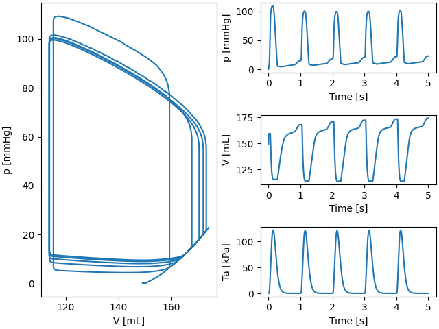
Fig. 2 Pressure volume loop for the LV.#
References#
Sander Land, So-Jin Park-Holohan, Nicolas P Smith, Cristobal G Dos Remedios, Jonathan C Kentish, and Steven A Niederer. A model of cardiac contraction based on novel measurements of tension development in human cardiomyocytes. Journal of molecular and cellular cardiology, 106:68–83, 2017.
Francesco Regazzoni, Matteo Salvador, Pasquale Claudio Africa, Marco Fedele, Luca Dedè, and Alfio Quarteroni. A cardiac electromechanical model coupled with a lumped-parameter model for closed-loop blood circulation. Journal of Computational Physics, 457:111083, 2022.
Jakub Tomek, Alfonso Bueno-Orovio, Elisa Passini, Xin Zhou, Ana Minchole, Oliver Britton, Chiara Bartolucci, Stefano Severi, Alvin Shrier, Laszlo Virag, and others. Development, calibration, and validation of a novel human ventricular myocyte model in health, disease, and drug block. Elife, 8:e48890, 2019.