BiV ellipsoid coupled to a 0D circulatory model and a 0D cell model#
This example extends the LV-only coupling example to a Bi-Ventricular (BiV) geometry. It couples a 3D BiV finite element model with a 0D closed-loop circulation model and a 0D cellular electrophysiology model.
Key Differences from LV Example#
Geometry: We use an idealized BiV geometry containing two cavities: Left Ventricle (LV) and Right Ventricle (RV).
Volume Constraints: We now have two volume constraints, one for each cavity (\(V_{LV}\) and \(V_{RV}\)).
Coupling Interface: The coupling function must accept target volumes for both ventricles and return pressures for both.
Models#
Mechanics: 3D BiV model with Holzapfel-Ogden material, active stress, and cavity volume constraints.
Circulation: [Regazzoni et al. 2022] lumped-parameter model. We replace both the 0D LV and RV chambers with our 3D model.
Cell Model: TorOrd-Land model for active tension generation.
from pathlib import Path
import circulation
from dolfinx import log
import matplotlib.pyplot as plt
from matplotlib.gridspec import GridSpec
import matplotlib.pyplot as plt
import numpy as np
import gotranx
import io4dolfinx
import cardiac_geometries
import cardiac_geometries.geometry
import pulse
circulation.log.setup_logging(logging.INFO)
logger = logging.getLogger("pulse")
comm = MPI.COMM_WORLD
geodir = Path("biv_ellipsoid-time-dependent")
if not geodir.exists():
    comm.barrier()
    cardiac_geometries.mesh.biv_ellipsoid(
        outdir=geodir,
        create_fibers=True,
        fiber_space="Quadrature_6",
        comm=comm,
        char_length=1.0,
        fiber_angle_epi=-60,
        fiber_angle_endo=60,
    )
Info    : Reading 'biv_ellipsoid-time-dependent/biv_ellipsoid.msh'...
Info    : 42 entities
Info    : 315 nodes
Info    : 1551 elements
Info    : Done reading 'biv_ellipsoid-time-dependent/biv_ellipsoid.msh'
                    INFO     INFO:ldrb.ldrb:Compute scalar laplacian solutions with the markers:                                                                                             ldrb.py:619
                             lv: [3]
                             rv: [4]
                             epi: [1]
                             base: [2]
# If the folder already exist, then we just load the geometry
geo = cardiac_geometries.geometry.Geometry.from_folder(
    comm=comm,
    folder=geodir,
)
# Scale the geometry to meters and adjust the size so that LV and RV volumes are reasonable
geo.mesh.geometry.x[:] *= 1.6e-2
[06/30/26 21:20:26] INFO INFO:cardiac_geometries.geometry:Reading geometry from biv_ellipsoid-time-dependent geometry.py:518
geometry = pulse.HeartGeometry.from_cardiac_geometries(
    geo, metadata={"quadrature_degree": 6},
)
Next we create the material object, and we will use the transversely isotropic version of the Holzapfel Ogden model
material_params = pulse.HolzapfelOgden.transversely_isotropic_parameters()
# material_params = pulse.HolzapfelOgden.orthotropic_parameters()
material = pulse.HolzapfelOgden(f0=geo.f0, s0=geo.s0, **material_params)  # type: ignore
We use an active stress approach with 30% transverse active stress (see pulse.active_stress.transversely_active_stress())
Ta = pulse.Variable(
    dolfinx.fem.Constant(geometry.mesh, dolfinx.default_scalar_type(0.0)), "kPa",
)
active_model = pulse.ActiveStress(geo.f0, activation=Ta)
We use an incompressible model
and assembles the CardiacModel
model = pulse.CardiacModel(
    material=material,
    active=active_model,
    compressibility=comp_model,
    # viscoelasticity=viscoeleastic_model,
)
alpha_epi = pulse.Variable(
    dolfinx.fem.Constant(geometry.mesh, dolfinx.default_scalar_type(1e6)),
    "Pa / m",
)
robin_epi = pulse.RobinBC(value=alpha_epi, marker=geometry.markers["EPI"][0])
alpha_base = pulse.Variable(
    dolfinx.fem.Constant(geometry.mesh, dolfinx.default_scalar_type(1e5)),
    "Pa / m",
)
robin_base = pulse.RobinBC(value=alpha_base, marker=geometry.markers["BASE"][0])
lvv_initial = geo.mesh.comm.allreduce(geometry.volume("LV"), op=MPI.SUM)
lv_volume = dolfinx.fem.Constant(
    geometry.mesh, dolfinx.default_scalar_type(lvv_initial),
)
lv_cavity = pulse.problem.Cavity(marker="LV", volume=lv_volume)
rvv_initial = geo.mesh.comm.allreduce(geometry.volume("RV"), op=MPI.SUM)
rv_volume = dolfinx.fem.Constant(
    geometry.mesh, dolfinx.default_scalar_type(rvv_initial),
)
rv_cavity = pulse.problem.Cavity(marker="RV", volume=rv_volume)
parameters = {"base_bc": pulse.problem.BaseBC.free, "mesh_unit": "m"}
outdir = Path("biv_ellipsoid_time_dependent_circulation_static")
bcs = pulse.BoundaryConditions(robin=(robin_epi, robin_base))
problem = pulse.problem.StaticProblem(
    model=model, geometry=geometry, bcs=bcs, cavities=cavities, parameters=parameters,
)
outdir.mkdir(exist_ok=True)
Now we can solve the problem
# log.set_log_level(log.LogLevel.INFO)
problem.solve()
True
dt = 0.001
times = np.arange(0.0, 1.0, dt)
ode = gotranx.load_ode("TorOrdLand.ode")
ode = ode.remove_singularities()
code = gotranx.cli.gotran2py.get_code(
    ode,
    scheme=[gotranx.schemes.Scheme.generalized_rush_larsen],
    shape=gotranx.codegen.base.Shape.single,
)
Path("TorOrdLand.py").write_text(code)
import TorOrdLand
2026-06-30 21:20:46 [info ] Load ode TorOrdLand.ode
2026-06-30 21:20:47 [info ] Num states 52
2026-06-30 21:20:47 [info ] Num parameters 140
TorOrdLand_model = TorOrdLand.__dict__
Ta_index = TorOrdLand_model["monitor_index"]("Ta")
y = TorOrdLand_model["init_state_values"]()
# Get initial parameter values
p = TorOrdLand_model["init_parameter_values"]()
import numba
fgr = numba.njit(TorOrdLand_model["generalized_rush_larsen"])
mon = numba.njit(TorOrdLand_model["monitor_values"])
V_index = TorOrdLand_model["state_index"]("v")
Ca_index = TorOrdLand_model["state_index"]("cai")
# Time in milliseconds
dt_cell = 0.1
state_file = outdir / "state.npy"
if not state_file.is_file():
@numba.jit(nopython=True)
def solve_beat(times, states, dt, p, V_index, Ca_index, Vs, Cais, Tas):
for i, ti in enumerate(times):
states[:] = fgr(states, ti, dt, p)
Vs[i] = states[V_index]
Cais[i] = states[Ca_index]
monitor = mon(ti, states, p)
Tas[i] = monitor[Ta_index]
# Time in milliseconds
nbeats = 200
T = 1000.00
times = np.arange(0, T, dt_cell)
all_times = np.arange(0, T * nbeats, dt_cell)
Vs = np.zeros(len(times) * nbeats)
Cais = np.zeros(len(times) * nbeats)
Tas = np.zeros(len(times) * nbeats)
logger.debug(f"Starting to solve {nbeats} beats of the cell model")
for beat in range(nbeats):
logger.debug(f"Solving beat {beat}")
V_tmp = Vs[beat * len(times) : (beat + 1) * len(times)]
Cai_tmp = Cais[beat * len(times) : (beat + 1) * len(times)]
Ta_tmp = Tas[beat * len(times) : (beat + 1) * len(times)]
solve_beat(times, y, dt_cell, p, V_index, Ca_index, V_tmp, Cai_tmp, Ta_tmp)
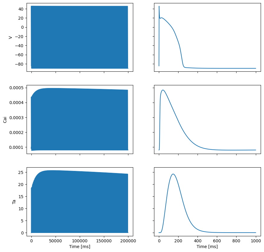
fig, ax = plt.subplots(3, 2, sharex="col", sharey="row", figsize=(10, 10))
ax[0, 0].plot(all_times, Vs)
ax[1, 0].plot(all_times, Cais)
ax[2, 0].plot(all_times, Tas)
ax[0, 1].plot(times, Vs[-len(times) :])
ax[1, 1].plot(times, Cais[-len(times) :])
ax[2, 1].plot(times, Tas[-len(times) :])
ax[0, 0].set_ylabel("V")
ax[1, 0].set_ylabel("Cai")
ax[2, 0].set_ylabel("Ta")
ax[2, 0].set_xlabel("Time [ms]")
ax[2, 1].set_xlabel("Time [ms]")
fig.savefig(outdir / "Ta_ORdLand.png")
if comm.rank == 0:
np.save(state_file, y)
np.save(outdir / "ode_times.npy", times)
np.save(outdir / "ode_Tas.npy", Tas[-len(times) :]) # Save only last beat
comm.barrier()
y = np.load(state_file)
ode_ts = np.load(outdir / "ode_times.npy")
ode_Tas = np.load(outdir / "ode_Tas.npy")
num_beats = 5
BCL = 1.0
@lru_cache
def get_activation(t: float):
    return np.interp((t % BCL) * 1000, ode_ts, ode_Tas) * 5.0
vtx = dolfinx.io.VTXWriter(
    geometry.mesh.comm, f"{outdir}/displacement.bp", [problem.u], engine="BP4",
)
vtx.write(0.0)
ts = np.arange(0.0, num_beats * BCL, dt)
Tas = [get_activation(ti) for ti in ts]
filename = Path("function_checkpoint.bp")
io4dolfinx.write_mesh(filename, geometry.mesh)
Ta_history: list[float] = []
def callback(model, i: int, t: float, save=True):
    Ta_history.append(get_activation(t))
    if save and i % 10 == 0:
        io4dolfinx.write_function(filename, problem.u, time=t, name="displacement")
        vtx.write(t)

        fig = plt.figure(layout="constrained", figsize=(12, 8))
        gs = GridSpec(3, 4, figure=fig)
        ax1 = fig.add_subplot(gs[:, 0])
        ax2 = fig.add_subplot(gs[:, 1])
        ax3 = fig.add_subplot(gs[0, 2])
        ax4 = fig.add_subplot(gs[1, 2])
        ax5 = fig.add_subplot(gs[0, 3])
        ax6 = fig.add_subplot(gs[1, 3])
        ax7 = fig.add_subplot(gs[2, 2:])

        ax1.plot(model.history["V_LV"][: i + 1], model.history["p_LV"][: i + 1])
        ax1.set_xlabel("LVV [mL]")
        ax1.set_ylabel("LVP [mmHg]")

        ax2.plot(model.history["V_RV"][: i + 1], model.history["p_RV"][: i + 1])
        ax2.set_xlabel("RVV [mL]")
        ax2.set_ylabel("RVP [mmHg]")

        ax3.plot(model.history["time"][: i + 1], model.history["p_LV"][: i + 1])
        ax3.set_ylabel("LVP [mmHg]")
        ax4.plot(model.history["time"][: i + 1], model.history["V_LV"][: i + 1])
        ax4.set_ylabel("LVV [mL]")

        ax5.plot(model.history["time"][: i + 1], model.history["p_RV"][: i + 1])
        ax5.set_ylabel("RVP [mmHg]")
        ax6.plot(model.history["time"][: i + 1], model.history["V_RV"][: i + 1])
        ax6.set_ylabel("RVV [mL]")

        ax7.plot(model.history["time"][: i + 1], Ta_history[: i + 1])
        ax7.set_ylabel("Ta [kPa]")

        for axi in [ax3, ax4, ax5, ax6, ax7]:
            axi.set_xlabel("Time [s]")

        fig.savefig(outdir / "pv_loop_incremental.png")
        plt.close(fig)
5. Coupling Function: 0D \(\rightarrow\) 3D (BiV)#
This function handles the interface for both ventricles.
Input: Circulation model provides target volumes \(V_{LV}\) and \(V_{RV}\), and time \(t\).
Active State: We get \(T_a(t)\) from the cell model.
Solve 3D:
Update
Taactive tension.Update both
lv_volumeandrv_volumeconstraint values.Solve the static equilibrium problem.
Output: We retrieve the Lagrange multipliers for both LV and RV cavities (indices 0 and 1 in
problem.cavity_pressures), convert them to mmHg, and return them.
def p_BiV_func(V_LV, V_RV, t):
    logger.debug("Calculating pressure at time %f", t)
    value = get_activation(t)
    logger.debug("Time %f Activation %f", t, value)

    logger.debug(f"Time{t} with activation: {value}")
    Ta.assign(value)
    lv_volume.value = V_LV * 1e-6
    rv_volume.value = V_RV * 1e-6
    problem.solve()

    lv_pendo_mmHg = circulation.units.kPa_to_mmHg(
        problem.cavity_pressures[0].x.array[0] * 1e-3,
    )
    rv_pendo_mmHg = circulation.units.kPa_to_mmHg(
        problem.cavity_pressures[1].x.array[0] * 1e-3,
    )

    return lv_pendo_mmHg, rv_pendo_mmHg
mL = circulation.units.ureg("mL")
add_units = False
lvv_init = (
    geo.mesh.comm.allreduce(geometry.volume("LV", u=problem.u), op=MPI.SUM)
    * 1e6
    * 1.0
)  # Increase the volume by 5%
rvv_init = (
    geo.mesh.comm.allreduce(geometry.volume("RV", u=problem.u), op=MPI.SUM)
    * 1e6
    * 1.0
)  # Increase the volume by 5%
logger.info(f"Initial volume (LV): {lvv_init} mL and (RV): {rvv_init} mL")
init_state = {"V_LV": lvv_initial * 1e6 * mL, "V_RV": rvv_initial * 1e6 * mL}
[06/30/26 21:21:55] INFO INFO:pulse:Initial volume (LV): 115.85870257039467 mL and (RV): 66.34467873625714 mL 1307119509.py:13
circulation_model_3D = circulation.regazzoni2020.Regazzoni2020(
    add_units=add_units,
    callback=callback,
    p_BiV=p_BiV_func,
    verbose=True,
    comm=comm,
    outdir=outdir,
    initial_state=init_state,
)
# exit()
# Set end time for early stopping if running in CI
end_time = 2 * dt if os.getenv("CI") else None
circulation_model_3D.solve(
    num_beats=num_beats, initial_state=init_state, dt=dt, T=end_time,
)
circulation_model_3D.print_info()
                    INFO     INFO:circulation.base:                                                                                                                                          base.py:134
                                                    Circulation model parameters (Regazzoni2020)
                             ┏━━━━━━━━━━━━━━━━━━━━━━━━━━━━━━━━━━━━━━━┳━━━━━━━━━━━━━━━━━━━━━━━━━━━━━━━━━━━━━━━━━━━━━━━━━┓
                             ┃ Parameter                             ┃ Value                                           ┃
                             ┡━━━━━━━━━━━━━━━━━━━━━━━━━━━━━━━━━━━━━━━╇━━━━━━━━━━━━━━━━━━━━━━━━━━━━━━━━━━━━━━━━━━━━━━━━━┩
                             │ HR                                    │ 1.25 hertz                                      │
                             │ chambers.LA.EA                        │ 0.07 millimeter_Hg / milliliter                 │
                             │ chambers.LA.EB                        │ 0.18 millimeter_Hg / milliliter                 │
                             │ chambers.LA.TC                        │ 0.17 second                                     │
                             │ chambers.LA.TR                        │ 0.17 second                                     │
                             │ chambers.LA.tC                        │ 0.9 second                                      │
                             │ chambers.LA.V0                        │ 4.0 milliliter                                  │
                             │ chambers.LV.EA                        │ 4.482 millimeter_Hg / milliliter                │
                             │ chambers.LV.EB                        │ 0.17 millimeter_Hg / milliliter                 │
                             │ chambers.LV.TC                        │ 0.25 second                                     │
                             │ chambers.LV.TR                        │ 0.4 second                                      │
                             │ chambers.LV.tC                        │ 0.1 second                                      │
                             │ chambers.LV.V0                        │ 42.0 milliliter                                 │
                             │ chambers.RA.EA                        │ 0.06 millimeter_Hg / milliliter                 │
                             │ chambers.RA.EB                        │ 0.07 millimeter_Hg / milliliter                 │
                             │ chambers.RA.TC                        │ 0.17 second                                     │
                             │ chambers.RA.TR                        │ 0.17 second                                     │
                             │ chambers.RA.tC                        │ 0.9 second                                      │
                             │ chambers.RA.V0                        │ 4.0 milliliter                                  │
                             │ chambers.RV.EA                        │ 0.2 millimeter_Hg / milliliter                  │
                             │ chambers.RV.EB                        │ 0.029 millimeter_Hg / milliliter                │
                             │ chambers.RV.TC                        │ 0.25 second                                     │
                             │ chambers.RV.TR                        │ 0.4 second                                      │
                             │ chambers.RV.tC                        │ 0.1 second                                      │
                             │ chambers.RV.V0                        │ 16.0 milliliter                                 │
                             │ valves.MV.Rmin                        │ 0.0075 millimeter_Hg * second / milliliter      │
                             │ valves.MV.Rmax                        │ 75006.2 millimeter_Hg * second / milliliter     │
                             │ valves.AV.Rmin                        │ 0.0075 millimeter_Hg * second / milliliter      │
                             │ valves.AV.Rmax                        │ 75006.2 millimeter_Hg * second / milliliter     │
                             │ valves.TV.Rmin                        │ 0.0075 millimeter_Hg * second / milliliter      │
                             │ valves.TV.Rmax                        │ 75006.2 millimeter_Hg * second / milliliter     │
                             │ valves.PV.Rmin                        │ 0.0075 millimeter_Hg * second / milliliter      │
                             │ valves.PV.Rmax                        │ 75006.2 millimeter_Hg * second / milliliter     │
                             │ circulation.SYS.R_AR                  │ 0.733 millimeter_Hg * second / milliliter       │
                             │ circulation.SYS.C_AR                  │ 1.372 milliliter / millimeter_Hg                │
                             │ circulation.SYS.R_VEN                 │ 0.32 millimeter_Hg * second / milliliter        │
                             │ circulation.SYS.C_VEN                 │ 11.363 milliliter / millimeter_Hg               │
                             │ circulation.SYS.L_AR                  │ 0.005 millimeter_Hg * second ** 2 / milliliter  │
                             │ circulation.SYS.L_VEN                 │ 0.0005 millimeter_Hg * second ** 2 / milliliter │
                             │ circulation.PUL.R_AR                  │ 0.046 millimeter_Hg * second / milliliter       │
                             │ circulation.PUL.C_AR                  │ 20.0 milliliter / millimeter_Hg                 │
                             │ circulation.PUL.R_VEN                 │ 0.0015 millimeter_Hg * second / milliliter      │
                             │ circulation.PUL.C_VEN                 │ 16.0 milliliter / millimeter_Hg                 │
                             │ circulation.PUL.L_AR                  │ 0.0005 millimeter_Hg * second ** 2 / milliliter │
                             │ circulation.PUL.L_VEN                 │ 0.0005 millimeter_Hg * second ** 2 / milliliter │
                             │ circulation.external.start_withdrawal │ 0.0 second                                      │
                             │ circulation.external.end_withdrawal   │ 0.0 second                                      │
                             │ circulation.external.start_infusion   │ 0.0 second                                      │
                             │ circulation.external.end_infusion     │ 0.0 second                                      │
                             │ circulation.external.flow_withdrawal  │ 0.0 milliliter / second                         │
                             │ circulation.external.flow_infusion    │ 0.0 milliliter / second                         │
                             └───────────────────────────────────────┴─────────────────────────────────────────────────┘
                    INFO     INFO:circulation.base:                                                                                                                                          base.py:141
                                   Circulation model initial states
                                            (Regazzoni2020)
                             ┏━━━━━━━━━━━┳━━━━━━━━━━━━━━━━━━━━━━━━━━━━━━━┓
                             ┃ State     ┃ Value                         ┃
                             ┡━━━━━━━━━━━╇━━━━━━━━━━━━━━━━━━━━━━━━━━━━━━━┩
                             │ V_LA      │ 87.183 milliliter             │
                             │ V_LV      │ 115.85870257039467 milliliter │
                             │ V_RA      │ 86.833 milliliter             │
                             │ V_RV      │ 66.34467873625714 milliliter  │
                             │ p_AR_SYS  │ 87.675 millimeter_Hg          │
                             │ p_VEN_SYS │ 35.898 millimeter_Hg          │
                             │ p_AR_PUL  │ 19.545 millimeter_Hg          │
                             │ p_VEN_PUL │ 15.004 millimeter_Hg          │
                             │ Q_AR_SYS  │ 71.104 milliliter / second    │
                             │ Q_VEN_SYS │ 94.039 milliliter / second    │
                             │ Q_AR_PUL  │ 94.084 milliliter / second    │
                             │ Q_VEN_PUL │ 473.279 milliliter / second   │
                             └───────────┴───────────────────────────────┘
                    INFO     INFO:circulation.base:                                                                                                                                          base.py:512
                                                                                        Volumes
                             ┏━━━━━━━━┳━━━━━━━━━┳━━━━━━━━┳━━━━━━━━┳━━━━━━━━━━┳━━━━━━━━━━━┳━━━━━━━━━━┳━━━━━━━━━━━┳━━━━━━━━━┳━━━━━━━━━┳━━━━━━━━━┳━━━━━━━━━━┓
                             ┃ V_LA   ┃ V_LV    ┃ V_RA   ┃ V_RV   ┃ V_AR_SYS ┃ V_VEN_SYS ┃ V_AR_PUL ┃ V_VEN_PUL ┃ Heart   ┃ SYS     ┃ PUL     ┃ Total    ┃
                             ┡━━━━━━━━╇━━━━━━━━━╇━━━━━━━━╇━━━━━━━━╇━━━━━━━━━━╇━━━━━━━━━━━╇━━━━━━━━━━╇━━━━━━━━━━━╇━━━━━━━━━╇━━━━━━━━━╇━━━━━━━━━╇━━━━━━━━━━┩
                             │ 85.728 │ 117.787 │ 86.183 │ 67.088 │ 120.219  │ 407.886   │ 390.806  │ 239.685   │ 356.787 │ 528.105 │ 630.491 │ 1515.382 │
                             └────────┴─────────┴────────┴────────┴──────────┴───────────┴──────────┴───────────┴─────────┴─────────┴─────────┴──────────┘

                                                                Pressures
                             ┏━━━━━━━━┳━━━━━━━┳━━━━━━━┳━━━━━━━┳━━━━━━━━━━┳━━━━━━━━━━━┳━━━━━━━━━━┳━━━━━━━━━━━┓
                             ┃ p_LA   ┃ p_LV  ┃ p_RA  ┃ p_RV  ┃ p_AR_SYS ┃ p_VEN_SYS ┃ p_AR_PUL ┃ p_VEN_PUL ┃
                             ┡━━━━━━━━╇━━━━━━━╇━━━━━━━╇━━━━━━━╇━━━━━━━━━━╇━━━━━━━━━━━╇━━━━━━━━━━╇━━━━━━━━━━━┩
                             │ 14.973 │ 0.494 │ 5.798 │ 0.204 │ 87.623   │ 35.896    │ 19.540   │ 14.980    │
                             └────────┴───────┴───────┴───────┴──────────┴───────────┴──────────┴───────────┘

                                                                     Flows
                             ┏━━━━━━━━━━┳━━━━━━━━┳━━━━━━━━━┳━━━━━━━━┳━━━━━━━━━━┳━━━━━━━━━━━┳━━━━━━━━━━┳━━━━━━━━━━━┓
                             ┃ Q_MV     ┃ Q_AV   ┃ Q_TV    ┃ Q_PV   ┃ Q_AR_SYS ┃ Q_VEN_SYS ┃ Q_AR_PUL ┃ Q_VEN_PUL ┃
                             ┡━━━━━━━━━━╇━━━━━━━━╇━━━━━━━━━╇━━━━━━━━╇━━━━━━━━━━╇━━━━━━━━━━━╇━━━━━━━━━━╇━━━━━━━━━━━┩
                             │ 1928.293 │ -0.001 │ 743.777 │ -0.000 │ 71.036   │ 94.053    │ 94.510   │ 471.921   │
                             └──────────┴────────┴─────────┴────────┴──────────┴───────────┴──────────┴───────────┘
[06/30/26 21:22:00] INFO     INFO:circulation.base:                                                                                                                                          base.py:512
                                                                                        Volumes
                             ┏━━━━━━━━┳━━━━━━━━━┳━━━━━━━━┳━━━━━━━━┳━━━━━━━━━━┳━━━━━━━━━━━┳━━━━━━━━━━┳━━━━━━━━━━━┳━━━━━━━━━┳━━━━━━━━━┳━━━━━━━━━┳━━━━━━━━━━┓
                             ┃ V_LA   ┃ V_LV    ┃ V_RA   ┃ V_RV   ┃ V_AR_SYS ┃ V_VEN_SYS ┃ V_AR_PUL ┃ V_VEN_PUL ┃ Heart   ┃ SYS     ┃ PUL     ┃ Total    ┃
                             ┡━━━━━━━━╇━━━━━━━━━╇━━━━━━━━╇━━━━━━━━╇━━━━━━━━━━╇━━━━━━━━━━━╇━━━━━━━━━━╇━━━━━━━━━━━╇━━━━━━━━━╇━━━━━━━━━╇━━━━━━━━━╇━━━━━━━━━━┩
                             │ 84.359 │ 119.628 │ 85.573 │ 67.792 │ 120.148  │ 407.863   │ 390.711  │ 239.307   │ 357.353 │ 528.011 │ 630.019 │ 1515.382 │
                             └────────┴─────────┴────────┴────────┴──────────┴───────────┴──────────┴───────────┴─────────┴─────────┴─────────┴──────────┘

                                                                Pressures
                             ┏━━━━━━━━┳━━━━━━━┳━━━━━━━┳━━━━━━━┳━━━━━━━━━━┳━━━━━━━━━━━┳━━━━━━━━━━┳━━━━━━━━━━━┓
                             ┃ p_LA   ┃ p_LV  ┃ p_RA  ┃ p_RV  ┃ p_AR_SYS ┃ p_VEN_SYS ┃ p_AR_PUL ┃ p_VEN_PUL ┃
                             ┡━━━━━━━━╇━━━━━━━╇━━━━━━━╇━━━━━━━╇━━━━━━━━━━╇━━━━━━━━━━━╇━━━━━━━━━━╇━━━━━━━━━━━┩
                             │ 14.711 │ 0.889 │ 5.753 │ 0.457 │ 87.571   │ 35.894    │ 19.536   │ 14.957    │
                             └────────┴───────┴───────┴───────┴──────────┴───────────┴──────────┴───────────┘

                                                                     Flows
                             ┏━━━━━━━━━━┳━━━━━━━━┳━━━━━━━━━┳━━━━━━━━┳━━━━━━━━━━┳━━━━━━━━━━━┳━━━━━━━━━━┳━━━━━━━━━━━┓
                             ┃ Q_MV     ┃ Q_AV   ┃ Q_TV    ┃ Q_PV   ┃ Q_AR_SYS ┃ Q_VEN_SYS ┃ Q_AR_PUL ┃ Q_VEN_PUL ┃
                             ┡━━━━━━━━━━╇━━━━━━━━╇━━━━━━━━━╇━━━━━━━━╇━━━━━━━━━━╇━━━━━━━━━━━╇━━━━━━━━━━╇━━━━━━━━━━━┩
                             │ 1840.775 │ -0.001 │ 703.949 │ -0.000 │ 70.967   │ 94.146    │ 94.935   │ 471.044   │
                             └──────────┴────────┴─────────┴────────┴──────────┴───────────┴──────────┴───────────┘
                    INFO     INFO:circulation.base:                                                                                                                                          base.py:512
                                                                                        Volumes
                             ┏━━━━━━━━┳━━━━━━━━━┳━━━━━━━━┳━━━━━━━━┳━━━━━━━━━━┳━━━━━━━━━━━┳━━━━━━━━━━┳━━━━━━━━━━━┳━━━━━━━━━┳━━━━━━━━━┳━━━━━━━━━┳━━━━━━━━━━┓
                             ┃ V_LA   ┃ V_LV    ┃ V_RA   ┃ V_RV   ┃ V_AR_SYS ┃ V_VEN_SYS ┃ V_AR_PUL ┃ V_VEN_PUL ┃ Heart   ┃ SYS     ┃ PUL     ┃ Total    ┃
                             ┡━━━━━━━━╇━━━━━━━━━╇━━━━━━━━╇━━━━━━━━╇━━━━━━━━━━╇━━━━━━━━━━━╇━━━━━━━━━━╇━━━━━━━━━━━╇━━━━━━━━━╇━━━━━━━━━╇━━━━━━━━━╇━━━━━━━━━━┩
                             │ 84.359 │ 119.628 │ 85.573 │ 67.792 │ 120.148  │ 407.863   │ 390.711  │ 239.307   │ 357.353 │ 528.011 │ 630.019 │ 1515.382 │
                             └────────┴─────────┴────────┴────────┴──────────┴───────────┴──────────┴───────────┴─────────┴─────────┴─────────┴──────────┘

                                                                Pressures
                             ┏━━━━━━━━┳━━━━━━━┳━━━━━━━┳━━━━━━━┳━━━━━━━━━━┳━━━━━━━━━━━┳━━━━━━━━━━┳━━━━━━━━━━━┓
                             ┃ p_LA   ┃ p_LV  ┃ p_RA  ┃ p_RV  ┃ p_AR_SYS ┃ p_VEN_SYS ┃ p_AR_PUL ┃ p_VEN_PUL ┃
                             ┡━━━━━━━━╇━━━━━━━╇━━━━━━━╇━━━━━━━╇━━━━━━━━━━╇━━━━━━━━━━━╇━━━━━━━━━━╇━━━━━━━━━━━┩
                             │ 14.711 │ 0.889 │ 5.753 │ 0.457 │ 87.571   │ 35.894    │ 19.536   │ 14.957    │
                             └────────┴───────┴───────┴───────┴──────────┴───────────┴──────────┴───────────┘

                                                                     Flows
                             ┏━━━━━━━━━━┳━━━━━━━━┳━━━━━━━━━┳━━━━━━━━┳━━━━━━━━━━┳━━━━━━━━━━━┳━━━━━━━━━━┳━━━━━━━━━━━┓
                             ┃ Q_MV     ┃ Q_AV   ┃ Q_TV    ┃ Q_PV   ┃ Q_AR_SYS ┃ Q_VEN_SYS ┃ Q_AR_PUL ┃ Q_VEN_PUL ┃
                             ┡━━━━━━━━━━╇━━━━━━━━╇━━━━━━━━━╇━━━━━━━━╇━━━━━━━━━━╇━━━━━━━━━━━╇━━━━━━━━━━╇━━━━━━━━━━━┩
                             │ 1840.775 │ -0.001 │ 703.949 │ -0.000 │ 70.967   │ 94.146    │ 94.935   │ 471.044   │
                             └──────────┴────────┴─────────┴────────┴──────────┴───────────┴──────────┴───────────┘
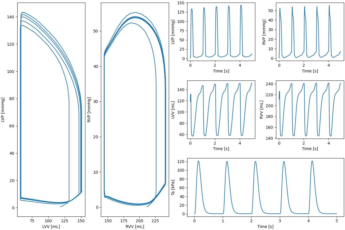
Fig. 3 Pressure volume loop for the BiV.#