Isometric Contraction and the Frank-Starling Mechanism#
In cardiac mechanics, the Frank-Starling mechanism describes how the heart inherently generates a greater active contraction force when it is subjected to a larger initial stretch (preload). At the cellular level, stretching the tissue moves the sarcomeres into a more optimal overlap configuration, allowing more myosin-actin cross-bridges to form.
In this tutorial, we will demonstrate this physiological phenomenon by conducting an isometric twitch experiment on a slab of myocardial tissue. We will:
Stretch the tissue to a specific length and lock the boundaries (isometric condition).
Measure the passive stress generated by stretching the hyperelastic collagen/myocardium matrix.
Activate the tissue and measure the additional active stress generated.
Compare a standard active stress model against our custom Frank-Starling model.
Mathematical Formulation of Active Stress#
In a standard active stress approach, the total 2nd Piola-Kirchhoff active stress acts purely along the reference fiber direction \(\mathbf{f}_0\) and is independent of stretch:
Where \(a(t)\) is the time-dependent activation scalar.
For the Frank-Starling mechanism, we introduce a stretch-dependent scalar multiplier \(g(\lambda)\). The total active First Piola-Kirchhoff stress (\(\mathbf{P}_{\text{act}}\)) evaluated by the FEM solver becomes:
Where \(\mathbf{F}\) is the deformation gradient, and \(\lambda = \sqrt{\mathbf{f}_0 \cdot (\mathbf{F}^T \mathbf{F} \mathbf{f}_0)}\) is the dynamic fiber stretch.
The multiplier \(g(\lambda)\) is defined as a piecewise function representing the ascending limb of the length-tension curve:
Where the slope \(m\) is calculated as:
1. Imports and Problem Setup#
First, we import the necessary modules. We use pulse for the mechanics framework, dolfinx for the finite element backend, mpi4py for parallel execution, and matplotlib for plotting our final results.
from mpi4py import MPI
import dolfinx
import pulse
import numpy as np
import ufl
import matplotlib.pyplot as plt
from scifem import evaluate_function
2. Defining the Isometric Twitch Experiment#
We define a function that takes a prescribed pre-stretch (in mm) and an active twitch tension (in kPa). It will stretch a 10x1x1 mm block of tissue, lock it in place, and then apply the active tension.
We include a boolean flag use_frank_starling to easily toggle between the standard active stress model and our stretch-dependent model.
def run_isometric_twitch(pre_stretch_mm: float, twitch_activation: float, use_frank_starling: bool = True):
    """
    Runs an isometric contraction on a 10x1x1 slab.
    1. Stretches the right face by `pre_stretch_mm` and locks it.
    2. Applies `twitch_activation` (kPa) to the active model.
    3. Returns the average passive and active fiber stresses.
    """
    # Create a 10 x 1 x 1 mm slab mesh
    L = 10.0
    mesh = dolfinx.mesh.create_box(
        MPI.COMM_WORLD,
        [[0.0, 0.0, 0.0], [L, 1.0, 1.0]],
        [10, 2, 2],
    )

    # Define microstructure (fibers aligned with the X-axis)
    f0 = dolfinx.fem.Constant(mesh, dolfinx.default_scalar_type((1.0, 0.0, 0.0)))
    s0 = dolfinx.fem.Constant(mesh, dolfinx.default_scalar_type((0.0, 1.0, 0.0)))

    # Trackers for active tension
    Ta = pulse.Variable(
        dolfinx.fem.Constant(mesh, dolfinx.default_scalar_type(0.0)), "kPa",
    )

    # Set up the passive material model
    material_params = pulse.HolzapfelOgden.transversely_isotropic_parameters()
    passive_model = pulse.HolzapfelOgden(
        f0=f0, s0=s0, **material_params,
    )

    # Toggle between the Frank-Starling model and the standard Active Stress model
    if not use_frank_starling:
        active_model = pulse.ActiveStress(f0=f0, activation=Ta)
    else:
        active_model = pulse.FrankStarlingActiveStress(f0=f0, activation=Ta)

    # Combine into a fully compressible cardiac model
    model = pulse.CardiacModel(
        material=passive_model,
        active=active_model,
        compressibility=pulse.Compressible2(),
    )

    # --- Geometry and Boundary Conditions ---
    boundaries = [
        pulse.Marker(name="X0", marker=1, dim=2, locator=lambda x: np.isclose(x[0], 0)),
        pulse.Marker(name="X1", marker=2, dim=2, locator=lambda x: np.isclose(x[0], L)),
    ]

    geo = pulse.Geometry(
        mesh=mesh,
        boundaries=boundaries,
        metadata={"quadrature_degree": 4},
    )

    def dirichlet_bc(
        V: dolfinx.fem.FunctionSpace,
    ) -> list[dolfinx.fem.bcs.DirichletBC]:
        mesh.topology.create_connectivity(mesh.topology.dim - 1, mesh.topology.dim)

        # 1. Lock the left face
        facets_fixed = geo.facet_tags.find(1)
        dofs = dolfinx.fem.locate_dofs_topological(V, 2, facets_fixed)
        u_fixed = dolfinx.fem.Function(V)
        u_fixed.x.array[:] = 0.0

        # 2. Stretch the right face in the X direction only
        facets_stretch = geo.facet_tags.find(2)
        V_x, _ = V.sub(0).collapse()
        dofs_x = dolfinx.fem.locate_dofs_topological((V.sub(0), V_x), 2, facets_stretch)

        u_stretch_x = dolfinx.fem.Function(V_x)
        u_stretch_x.x.array[:] = pre_stretch_mm

        return [
            dolfinx.fem.dirichletbc(u_stretch_x, dofs_x, V.sub(0)),
            dolfinx.fem.dirichletbc(u_fixed, dofs),
        ]

    bcs = pulse.BoundaryConditions(dirichlet=(dirichlet_bc,))

    # Set up the FEniCSx-Pulse mechanics problem
    parameters = {"mesh_unit": "mm"}
    problem = pulse.StaticProblem(model=model, geometry=geo, bcs=bcs, parameters=parameters)

    # CRITICAL: Register the displacement field for the Frank-Starling stretch tracking
    if use_frank_starling:
        active_model.register(problem.u)

    point = np.array([[L, 0.5, 0.5]])

    # --- Phase 1: Passive Pre-Stretch ---
    # Solve for the passive stretch equilibrium
    problem.solve()

    # Formulate the average fiber stress
    F = ufl.variable(ufl.grad(problem.u) + ufl.Identity(3))
    f = F * f0
    f_norm = f / ufl.sqrt(ufl.inner(f, f))

    # Integrate to find the domain volume
    volume = mesh.comm.allreduce(
        dolfinx.fem.assemble_scalar(dolfinx.fem.form(ufl.det(F) * geo.dx)), op=MPI.SUM,
    )

    # Integrate Cauchy stress projected onto the deformed fiber direction
    Tf = dolfinx.fem.form(ufl.inner(model.sigma(F) * f_norm, f_norm) * geo.dx)
    passive_force = mesh.comm.allreduce(dolfinx.fem.assemble_scalar(Tf), op=MPI.SUM) / volume

    # --- Phase 2: Active Twitch ---
    nsteps = 10
    for step in range(nsteps):
        # Ramp up activation over nsteps steps to aid Newton convergence
        Ta.assign(twitch_activation * (step + 1) / nsteps)
        problem.solve()

    # Calculate total stress after activation
    total_force = mesh.comm.allreduce(dolfinx.fem.assemble_scalar(Tf), op=MPI.SUM) / volume

    # Isolate the active contribution
    active_force = total_force - passive_force

    return passive_force, active_force
3. Running the Curve and Comparison#
We will loop over increasing amounts of stretch (from 0% up to 15%) and run the experiment twice per stretch: once with the standard active stress, and once with the Frank-Starling model.
twitch_force = 1.0 # kPa of active baseline tension

# Test stretches from 0 mm (0%) up to 1.5 mm (15%)
stretch_amounts = [0.0, 0.25, 0.5, 0.75, 1.0, 1.25, 1.5]
strain_pcts = [(s / 10.0) * 100 for s in stretch_amounts]

passive_stresses = []
active_stresses_std = []
active_stresses_fs = []

print(f"{'Stretch (%)':>12} | {'Passive Stress':>18} | {'Std Active Stress':>20} | {'FS Active Stress':>20}")
print("-" * 78)

for s, pct in zip(stretch_amounts, strain_pcts):
    # 1. Run Standard Model
    p_force, a_force_std = run_isometric_twitch(s, twitch_force, use_frank_starling=False)

    # 2. Run Frank-Starling Model
    _, a_force_fs = run_isometric_twitch(s, twitch_force, use_frank_starling=True)

    # Store results
    passive_stresses.append(p_force)
    active_stresses_std.append(a_force_std)
    active_stresses_fs.append(a_force_fs)

    print(f"{pct:12.2f} | {p_force:18.4f} | {a_force_std:20.4f} | {a_force_fs:20.4f}")
 Stretch (%) |     Passive Stress |    Std Active Stress |     FS Active Stress
------------------------------------------------------------------------------
0.00 | 0.0000 | 666.6667 | 333.3333
2.50 | 369.3137 | 700.9067 | 410.5990
5.00 | 840.7423 | 735.8393 | 494.1016
7.50 | 1546.8966 | 771.3395 | 583.7690
10.00 | 2755.5774 | 807.1158 | 679.2050
12.50 | 5069.9621 | 842.4616 | 779.0904
15.00 | 9921.8714 | 875.7425 | 869.0698
4. Plotting the Results#
While a table is useful, plotting the results makes the physiological phenomenon instantly clear. We will use matplotlib to plot the Active Stress (comparing both models) on the left axis, and the Passive hyperelastic stress on the right axis.
fig, ax1 = plt.subplots(figsize=(9, 6))

# Plot Active Stresses on the primary y-axis
ax1.set_xlabel('Stretch (%)', fontsize=12)
ax1.set_ylabel('Active Stress (kPa)', color='tab:blue', fontsize=12)

ax1.plot(
    strain_pcts, active_stresses_fs, marker='o', linewidth=2, color='tab:blue',
    label='Frank-Starling Active Stress',
)
ax1.plot(
    strain_pcts, active_stresses_std, marker='s', linestyle='--', linewidth=2, color='tab:cyan',
    label='Standard Active Stress',
)

ax1.tick_params(axis='y', labelcolor='tab:blue')
ax1.grid(True, linestyle='--', alpha=0.6)

# Create a twin axis for the Passive Stress
ax2 = ax1.twinx()
ax2.set_ylabel('Passive Stress (kPa)', color='tab:red', fontsize=12)
ax2.plot(
    strain_pcts, passive_stresses, marker='^', linewidth=2, color='tab:red',
    label='Passive Stress (Holzapfel-Ogden)',
)
ax2.tick_params(axis='y', labelcolor='tab:red')

# Add legends
lines_1, labels_1 = ax1.get_legend_handles_labels()
lines_2, labels_2 = ax2.get_legend_handles_labels()
ax1.legend(lines_1 + lines_2, labels_1 + labels_2, loc='upper center', bbox_to_anchor=(0.5, -0.15), ncol=3)

plt.title('Isometric Contraction: Frank-Starling vs. Standard Active Stress', fontsize=14)
fig.tight_layout()
plt.show()
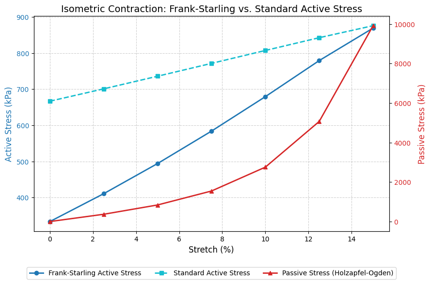
Conclusion#
The plot generated by the script perfectly illustrates two primary mechanics of the heart wall:
Exponential Passive Stiffening (Red Line): As the tissue is stretched past 10%, the collagen fibers un-crimp and become highly resistant to further stretch.
Frank-Starling Law (Dark Blue vs Light Blue): The standard model (dashed light blue) assumes a constant, 100% force capacity regardless of how compressed or stretched the sarcomeres are. The Frank-Starling model (solid dark blue) dynamically scales the force—starting lower at rest, and sharply climbing as the tissue stretches toward its optimal operating length.
Wait, why does the Standard Active Stress slightly increase? You might notice that the standard model’s active stress isn’t perfectly flat across stretches. This is actually physically and mathematically correct! In continuum mechanics, the active stress is defined in the reference configuration (2nd Piola-Kirchhoff stress). When we measure the true (Cauchy) stress in the deformed configuration, the solver applies a geometric “push-forward”.
As the tissue stretches, it physically narrows due to incompressibility (the Poisson effect). Because the cross-sectional area shrinks, the true stress (Force / Area) mechanically increases, even if the chemical contraction capability remained identical.
Thus, the Standard model increases purely due to kinematic/geometric stiffening, while the Frank-Starling model increases due to that same geometric effect plus the biological recruitment of more myosin-actin cross-bridges.