Using numba jit

In this example we will show how to use numba to jit compile the function, which will drastically speed up the computations. We will use the same model as in the previous example, but we will use the numba jit compiler to compile the functions. First we will import gotranx as well as a few other packages

import gotranx
import numba
from typing import Any
import numpy as np
import time
import matplotlib.pyplot as plt

For this tutorial we will use a rather large system of ODE which simulated the electromechanics in cardiac cells that are based on the O’Hara-Rudy model for electrophysiology and the Land model. You can download the model in .ode format here

We load the model using the load_ode() function

ode = gotranx.load_ode("ORdmm_Land.ode")

2024-11-05 20:05:51 [info     ] Load ode ORdmm_Land.ode       

2024-11-05 20:05:52 [info     ] Num states 48                 

2024-11-05 20:05:52 [info     ] Num parameters 139            

This set of ODE also contains some singularities that we can remove by replacing the expressions with piecewise functions. This is particularly important if we want to jit compile it because, while e.g division by zero in numpy only yields a warning, numba will crash if this happens. We can do this using the remove_singularities method

ode = ode.remove_singularities()

2024-11-05 20:05:54 [warning  ] Expression Isac_P_k is zero. Maybe you forgot to resolve the expression?

2024-11-05 20:05:54 [warning  ] Expression Isac_P_ns is zero. Maybe you forgot to resolve the expression?

Now we can generate code in python using the cli subpackage and the gotran2py module. We will also generate code for the generalized rush larsen scheme, and here we also explicitly set the shape of the output arrays to be single. By default, the function will check whether you run vectorized or not, and adapt the shape accordingly. However, such conditional statements are not supported by numba, so we need to explicitly set the shape to single.

code = gotranx.cli.gotran2py.get_code(
    ode, scheme=[gotranx.schemes.Scheme.generalized_rush_larsen], shape=gotranx.codegen.base.Shape.single,
)

Now we get back the code as a string. To actually execute this code you can either save it to a python file and import it, or you can execute it directly into some namespace (e.g a dictionary). Let’s do the latter

model: dict[str, Any] = {}
exec(code, model)

Now we can use the model dictionary to call the generated functions

y = model["init_state_values"]()
# Get initial parameter values
p = model["init_parameter_values"]()
# Set time step to 0.1 ms
dt = 0.1
# Simulate model for 1000 ms
t = np.arange(0, 1000, dt)
# Get the index of the membrane potential
V_index = model["state_index"]("v")
Ca_index = model["state_index"]("cai")
# Get the index of the active tension from the land model
Ta_index = model["monitor_index"]("Ta")
Istim_index = model["monitor_index"]("Istim")

Now we will compile the functions using numba. We will use the njit decorator to compile the functions. We will also compile the monitor_values function, which is used to monitor extract intermediate values such as Ta.

fgr = numba.njit(model["generalized_rush_larsen"])
mon = numba.njit(model["monitor_values"])

Let’s create a separate function to solve a single beat

@numba.njit
def solve_beat(times, states, dt, p, V_index, Ca_index, Vs, Cais, Tas):
    for i, ti in enumerate(times):
        states[:] = fgr(states, ti, dt, p)
        Vs[i] = states[V_index]
        Cais[i] = states[Ca_index]
        monitor = mon(ti, states, p)
        Tas[i] = monitor[Ta_index]

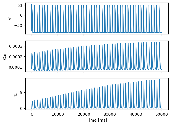
Let us simulate the model for 50 beats

nbeats = 50
T = 1000.00

t0 = time.perf_counter()
times = np.arange(0, T, 0.1)
all_times = np.arange(0, T * nbeats, 0.1)
Vs = np.zeros(len(times) * nbeats)
Cais = np.zeros(len(times) * nbeats)
Tas = np.zeros(len(times) * nbeats)
for beat in range(nbeats):
    V_tmp = Vs[beat * len(times) : (beat + 1) * len(times)]
    Cai_tmp = Cais[beat * len(times) : (beat + 1) * len(times)]
    Ta_tmp = Tas[beat * len(times) : (beat + 1) * len(times)]
    t1 = time.perf_counter()
    solve_beat(times, y, dt, p, V_index, Ca_index, V_tmp, Cai_tmp, Ta_tmp)
    print(f"Elapsed time (beat {beat + 1}): {time.perf_counter() - t1:.2f} s")
print(f"Elapsed time: {time.perf_counter() - t0:.2f} s")
# And plot the results

Elapsed time (beat 1): 14.81 s
Elapsed time (beat 2): 0.12 s
Elapsed time (beat 3): 0.11 s

Elapsed time (beat 4): 0.11 s
Elapsed time (beat 5): 0.11 s
Elapsed time (beat 6): 0.11 s
Elapsed time (beat 7): 0.11 s
Elapsed time (beat 8): 0.11 s

Elapsed time (beat 9): 0.11 s
Elapsed time (beat 10): 0.12 s
Elapsed time (beat 11): 0.11 s
Elapsed time (beat 12): 0.11 s

Elapsed time (beat 13): 0.12 s
Elapsed time (beat 14): 0.11 s
Elapsed time (beat 15): 0.11 s
Elapsed time (beat 16): 0.11 s
Elapsed time (beat 17): 0.11 s

Elapsed time (beat 18): 0.11 s
Elapsed time (beat 19): 0.11 s
Elapsed time (beat 20): 0.11 s
Elapsed time (beat 21): 0.11 s

Elapsed time (beat 22): 0.11 s
Elapsed time (beat 23): 0.11 s
Elapsed time (beat 24): 0.11 s
Elapsed time (beat 25): 0.11 s

Elapsed time (beat 26): 0.11 s
Elapsed time (beat 27): 0.11 s
Elapsed time (beat 28): 0.11 s
Elapsed time (beat 29): 0.11 s

Elapsed time (beat 30): 0.11 s
Elapsed time (beat 31): 0.11 s
Elapsed time (beat 32): 0.12 s
Elapsed time (beat 33): 0.11 s

Elapsed time (beat 34): 0.11 s
Elapsed time (beat 35): 0.11 s
Elapsed time (beat 36): 0.12 s
Elapsed time (beat 37): 0.11 s

Elapsed time (beat 38): 0.12 s
Elapsed time (beat 39): 0.11 s
Elapsed time (beat 40): 0.11 s
Elapsed time (beat 41): 0.11 s
Elapsed time (beat 42): 0.11 s

Elapsed time (beat 43): 0.12 s
Elapsed time (beat 44): 0.11 s
Elapsed time (beat 45): 0.11 s
Elapsed time (beat 46): 0.11 s
Elapsed time (beat 47): 0.11 s
Elapsed time (beat 48): 0.11 s

Elapsed time (beat 49): 0.11 s
Elapsed time (beat 50): 0.11 s
Elapsed time: 20.42 s

fig, ax = plt.subplots(3, 1, sharex=True)
ax[0].plot(all_times, Vs)
ax[1].plot(all_times, Cais)
ax[2].plot(all_times, Tas)
ax[0].set_ylabel("V")
ax[1].set_ylabel("Cai")
ax[2].set_ylabel("Ta")
ax[2].set_xlabel("Time [ms]")
plt.show()