Splitting an ODE into two sub-ODEs#
In some cases it might be useful to split an ODE into two separate ODEs, for example when you are modeling different dynamics and these are happening on different time scales. One example of this is when we model both the electrical and the mechanics of heart cells. We can model them within the same ODE, but you might want to embed the model inside a 3D tissue model, in which it is important to solve the dependent variables within the correct model (the PDEs for mechanics are typically more expensive to solve, so we want to solve them less frequently)
In this demo we will show how to split a model containing both the mechanical and the electrical models for a human heart cell.
We will use a rather large system of ODE which simulated the electromechanics in cardiac cells that are based on the O’Hara-Rudy model for electrophysiology and the Land model. You can download the model in .ode format here
First lets do the necessary imports
from pathlib import Path
import gotranx
from typing import Any
import numpy as np
import matplotlib.pyplot as plt
# And load the model
ode = gotranx.load_ode(Path.cwd() / "ORdmm_Land.ode")
2026-05-12 13:37:41 [info ] Load ode /home/runner/work/gotranx/gotranx/examples/split-ode/ORdmm_Land.ode
2026-05-12 13:37:42 [info ] Num states 48
2026-05-12 13:37:42 [info ] Num parameters 139
We will now pull out the component called "mechanics" and turn it into a separate ODE
mechanics_comp = ode.get_component("mechanics")
mechanics_ode = mechanics_comp.to_ode()
We can now find the remaining ODE by subtracting the full ODE from the mechanics ODE
ep_ode = ode - mechanics_comp
Now let us generate code for all the ODEs. We generate code for full model
code = gotranx.cli.gotran2py.get_code(
    ode,
    scheme=[gotranx.schemes.Scheme.forward_generalized_rush_larsen],
)
the electrophysiology model
code_ep = gotranx.cli.gotran2py.get_code(
    ep_ode,
    scheme=[gotranx.schemes.Scheme.forward_generalized_rush_larsen],
    missing_values=mechanics_ode.missing_variables,
)
and for the mechanics model
code_mechanics = gotranx.cli.gotran2py.get_code(
    mechanics_ode,
    scheme=[gotranx.schemes.Scheme.forward_generalized_rush_larsen],
    missing_values=ep_ode.missing_variables,
)
Now to actually get the models we can execute them into their own namespace (i.e dictionaries)
model: dict[str, Any] = {}
exec(code, model)
ep_model: dict[str, Any] = {}
exec(code_ep, ep_model)
mechanics_model: dict[str, Any] = {}
exec(code_mechanics, mechanics_model)
We set time step to 0.1 ms, and simulate model for 1000 ms
dt = 0.1
t = np.arange(0, 1000, dt)
Now we need to set up all variables
# Get the index of the membrane potential
V_index_ep = ep_model["state_index"]("v")
# Forward generalized rush larsen scheme for the electrophysiology model
fgr_ep = ep_model["forward_generalized_rush_larsen"]
# Monitor function for the electrophysiology model
mon_ep = ep_model["monitor_values"]
# Missing values function for the electrophysiology model
mv_ep = ep_model["missing_values"]
# Index of the calcium concentration
Ca_index_ep = ep_model["state_index"]("cai")
# Forward generalized rush larsen scheme for the mechanics model
fgr_mechanics = mechanics_model["forward_generalized_rush_larsen"]
# Monitor function for the mechanics model
mon_mechanics = mechanics_model["monitor_values"]
# Missing values function for the mechanics model
mv_mechanics = mechanics_model["missing_values"]
# Index of the active tension
Ta_index_mechanics = mechanics_model["monitor_index"]("Ta")
# Index of the J_TRPN
J_TRPN_index_mechanics = mechanics_model["monitor_index"]("J_TRPN")
# Forward generalized rush larsen scheme for the full model
fgr = model["forward_generalized_rush_larsen"]
# Monitor function for the full model
mon = model["monitor_values"]
# Index of the active tension for the full model
Ta_index = model["monitor_index"]("Ta")
# Index of the J_TRPN for the full model
J_TRPN_index = model["monitor_index"]("J_TRPN")
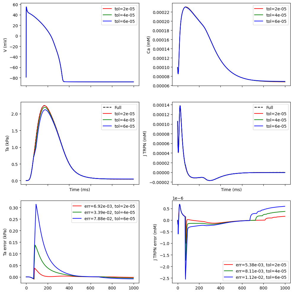
We will now see how many steps we need to ensure that the missing variables that are passed from the EP model to the mechanics model are below a certain tolerance. Lower tolerance will typically mean more steps, and we would like to see how the solution depends on how often we solve the ODE
# Tolerances to test for when to perform steps in the mechanics model
tols = [2e-5, 4e-5, 6e-5]
# Colors for the plots
colors = ["r", "g", "b", "c", "m"]
We create some arrays to store the results
# Create arrays to store the results
V_ep = np.zeros(len(t))
Ca_ep = np.zeros(len(t))
J_TRPN_full = np.zeros(len(t))
Ta_full = np.zeros(len(t))

Ta_mechanics = np.zeros(len(t))
J_TRPN_mechanics = np.zeros(len(t))
And we run the loop
fig, ax = plt.subplots(3, 2, sharex=True, figsize=(10, 10))
for j, (col, tol) in enumerate(zip(colors, tols)):
    # Get initial values from the EP model
    y_ep = ep_model["init_state_values"]()
    p_ep = ep_model["init_parameter_values"]()
    ep_missing_values = np.zeros(len(ep_ode.missing_variables))

    # Get initial values from the mechanics model
    y_mechanics = mechanics_model["init_state_values"]()
    p_mechanics = mechanics_model["init_parameter_values"]()
    mechanics_missing_values = np.zeros(len(mechanics_ode.missing_variables))

    # Get the initial values from the full model
    y = model["init_state_values"]()
    p = model["init_parameter_values"]()

    # Get the default values of the missing values
    # A little bit chicken and egg problem here, but in this specific case we know that the mechanics_missing_values is only the calcium concentration, which is a state variable and this doesn't require any additional information to be calculated.
    mechanics_missing_values[:] = mv_ep(0, y_ep, p_ep, ep_missing_values)
    ep_missing_values[:] = mv_mechanics(0, y_mechanics, p_mechanics, mechanics_missing_values)

    # We will store the previous missing values to check for convergence
    prev_mechanics_missing_values = np.zeros_like(mechanics_missing_values)
    prev_mechanics_missing_values[:] = mechanics_missing_values

    inds = []
    for i, ti in enumerate(t):
        # Forward step for the full model
        y[:] = fgr(y, ti, dt, p)
        monitor = mon(ti, y, p)
        J_TRPN_full[i] = monitor[J_TRPN_index]
        Ta_full[i] = monitor[Ta_index]

        # Forward step for the EP model
        y_ep[:] = fgr_ep(y_ep, ti, dt, p_ep, ep_missing_values)
        V_ep[i] = y_ep[V_index_ep]
        Ca_ep[i] = y_ep[Ca_index_ep]
        monitor_ep = mon_ep(ti, y_ep, p_ep, ep_missing_values)

        # Update missing values for the mechanics model
        mechanics_missing_values[:] = mv_ep(t, y_ep, p_ep, ep_missing_values)

        # Compute the change in the missing values
        change = np.linalg.norm(
            mechanics_missing_values - prev_mechanics_missing_values
        ) / np.linalg.norm(prev_mechanics_missing_values)

        # Check if the change is small enough to continue to the next time step
        if change < tol:
            # Very small change to just continue to next time step
            continue

        # Store the index of the time step where we performed a step
        inds.append(i)

        # Forward step for the mechanics model
        y_mechanics[:] = fgr_mechanics(y_mechanics, ti, dt, p_mechanics, mechanics_missing_values)
        monitor_mechanics = mon_mechanics(
            ti,
            y_mechanics,
            p_mechanics,
            mechanics_missing_values,
        )
        Ta_mechanics[i] = monitor_mechanics[Ta_index_mechanics]
        J_TRPN_mechanics[i] = monitor_mechanics[J_TRPN_index_mechanics]

        # Update missing values for the EP model
        ep_missing_values[:] = mv_mechanics(t, y_mechanics, p_mechanics, mechanics_missing_values)

        prev_mechanics_missing_values[:] = mechanics_missing_values

    # Plot the results
    print(f"Solved on {100 * len(inds) / len(t)}% of the time steps")
    inds = np.array(inds)

    ax[0, 0].plot(t, V_ep, color=col, label=f"tol={tol}")

    if j == 0:
        # Plot the full model with a dashed line only for the first run
        ax[1, 0].plot(t, Ta_full, color="k", linestyle="--", label="Full")
        ax[1, 1].plot(t, J_TRPN_full, color="k", linestyle="--", label="Full")

    ax[1, 0].plot(t[inds], Ta_mechanics[inds], color=col, label=f"tol={tol}")

    ax[0, 1].plot(t, Ca_ep, color=col, label=f"tol={tol}")

    ax[1, 1].plot(t[inds], J_TRPN_mechanics[inds], color=col, label=f"tol={tol}")

    err_Ta = np.linalg.norm(Ta_full[inds] - Ta_mechanics[inds]) / np.linalg.norm(Ta_mechanics)
    err_J_TRPN = np.linalg.norm(J_TRPN_full[inds] - J_TRPN_mechanics[inds]) / np.linalg.norm(
        J_TRPN_mechanics
    )
    ax[2, 0].plot(
        t[inds],
        Ta_full[inds] - Ta_mechanics[inds],
        label=f"err={err_Ta:.2e}, tol={tol}",
        color=col,
    )

    ax[2, 1].plot(
        t[inds],
        J_TRPN_full[inds] - J_TRPN_mechanics[inds],
        label=f"err={err_J_TRPN:.2e}, tol={tol}",
        color=col,
    )

    ax[1, 0].set_xlabel("Time (ms)")
    ax[1, 1].set_xlabel("Time (ms)")
    ax[0, 0].set_ylabel("V (mV)")
    ax[1, 0].set_ylabel("Ta (kPa)")
    ax[0, 1].set_ylabel("Ca (mM)")
    ax[1, 1].set_ylabel("J TRPN (mM)")

    ax[2, 0].set_ylabel("Ta error (kPa)")
    ax[2, 1].set_ylabel("J TRPN error (mM)")

    for axi in ax.flatten():
        axi.legend()

    fig.tight_layout()
plt.show()
<string>:641: RuntimeWarning: divide by zero encountered in scalar power
<string>:3111: RuntimeWarning: divide by zero encountered in scalar power
<string>:3116: RuntimeWarning: invalid value encountered in scalar divide
<string>:771: RuntimeWarning: divide by zero encountered in scalar power
<string>:776: RuntimeWarning: invalid value encountered in scalar divide
Solved on 87.39% of the time steps
Solved on 78.88% of the time steps
Solved on 73.15% of the time steps

