
Comparing Cross-Bridge Models: Land, Lewalle, RDQ18, RDQ20MF#
The previous four demos each ran the same isometric twitch experiment –
a 10x1x1 mm slab of Holzapfel-Ogden tissue, pre-stretched and locked, then
activated – with a different
crossbridge
force-generation model in the loop:
Land2017[LPHS+17] – three-state cross-bridge cycle, length-dependent activation via two curve-fitted gradients.Lewalle2024[LMCN24] – the same cross-bridge cycle, but length dependence replaced by a mechanistic myosin OFF-state force-feedback loop.RDQ18[RDedeQ18] – cooperative regulatory-unit (RU) kinetics with explicit filament overlap; no force-velocity effect (\(K_a \equiv 0\)).RDQ20MF[RDedeQ20] –RDQ18’s RU kinetics plus an explicit, velocity-dependent cross-bridge (XB) cycle (\(K_a \neq 0\)).
All four expose the same interface
(advance_step/get_active_tension/get_active_stiffness), so all four
plug into pulse.StabilizedActiveStress [RQ21]
identically. This demo
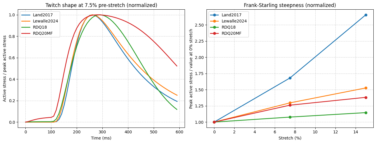
runs them side by side under matched conditions and compares what
actually differs: twitch shape, Frank-Starling steepness, and
absolute tension scale.
All four also reproduce the ad hoc FrankStarlingActiveStress idea from
the original frank_starling_twitch demo as
an emergent property of real sub-cellular kinetics rather than a fitted
multiplier – at the cost of a much heavier per-step computation and an
external dependency. Whether that trade is worth it depends on whether the
question being asked needs realistic twitch kinetics (rise time,
relaxation, calcium sensitivity) or only the steady-state length-tension
relationship, for which the phenomenological model is far cheaper.
from mpi4py import MPI

import dolfinx
import matplotlib.pyplot as plt
import numpy as np
import ufl
from crossbridge import RDQ18, RDQ20MF, Land2017, Lewalle2024, calcium_trace

import pulse
1. A model-agnostic isometric twitch runner#
The same coupling code as the individual demos, parameterized over which
crossbridge model class to drive it with.
def run_isometric_twitch(
    cell_cls,
    pre_stretch_mm: float,
    cell_kwargs: dict | None = None,
    calcium_kwargs: dict | None = None,
    t_end: float = 0.6,
    couple_dt: float = 1e-2,
):
    """
    Runs an isometric twitch on a 10x1x1 mm slab, driven by `cell_cls` (one
    of Land2017, Lewalle2024, RDQ18, RDQ20MF).

    Returns the passive fiber stress, and (time, active fiber stress,
    active stiffness) arrays.
    """
    cell_kwargs = cell_kwargs or {}
    calcium_kwargs = calcium_kwargs or {}

    L = 10.0
    mesh = dolfinx.mesh.create_box(
        MPI.COMM_WORLD,
        [[0.0, 0.0, 0.0], [L, 1.0, 1.0]],
        [10, 2, 2],
    )

    f0 = dolfinx.fem.Constant(mesh, dolfinx.default_scalar_type((1.0, 0.0, 0.0)))
    s0 = dolfinx.fem.Constant(mesh, dolfinx.default_scalar_type((0.0, 1.0, 0.0)))

    Ta = pulse.Variable(dolfinx.fem.Constant(mesh, dolfinx.default_scalar_type(0.0)), "kPa")
    Ka = pulse.Variable(dolfinx.fem.Constant(mesh, dolfinx.default_scalar_type(0.0)), "kPa")

    material_params = pulse.HolzapfelOgden.transversely_isotropic_parameters()
    passive_model = pulse.HolzapfelOgden(f0=f0, s0=s0, **material_params)
    active_model = pulse.StabilizedActiveStress(f0=f0, activation=Ta, active_stiffness=Ka)

    model = pulse.CardiacModel(
        material=passive_model,
        active=active_model,
        compressibility=pulse.Compressible2(),
    )

    boundaries = [
        pulse.Marker(name="X0", marker=1, dim=2, locator=lambda x: np.isclose(x[0], 0)),
        pulse.Marker(name="X1", marker=2, dim=2, locator=lambda x: np.isclose(x[0], L)),
    ]
    geo = pulse.Geometry(mesh=mesh, boundaries=boundaries, metadata={"quadrature_degree": 4})

    def dirichlet_bc(V: dolfinx.fem.FunctionSpace) -> list[dolfinx.fem.bcs.DirichletBC]:
        mesh.topology.create_connectivity(mesh.topology.dim - 1, mesh.topology.dim)

        facets_fixed = geo.facet_tags.find(1)
        dofs = dolfinx.fem.locate_dofs_topological(V, 2, facets_fixed)
        u_fixed = dolfinx.fem.Function(V)
        u_fixed.x.array[:] = 0.0

        facets_stretch = geo.facet_tags.find(2)
        V_x, _ = V.sub(0).collapse()
        dofs_x = dolfinx.fem.locate_dofs_topological((V.sub(0), V_x), 2, facets_stretch)
        u_stretch_x = dolfinx.fem.Function(V_x)
        u_stretch_x.x.array[:] = pre_stretch_mm

        return [
            dolfinx.fem.dirichletbc(u_stretch_x, dofs_x, V.sub(0)),
            dolfinx.fem.dirichletbc(u_fixed, dofs),
        ]

    bcs = pulse.BoundaryConditions(dirichlet=(dirichlet_bc,))
    parameters = {"mesh_unit": "mm"}
    problem = pulse.StaticProblem(model=model, geometry=geo, bcs=bcs, parameters=parameters)

    Vs = dolfinx.fem.functionspace(mesh, ("DG", 1))
    active_model.lmbda_prev = dolfinx.fem.Function(Vs)
    active_model.lmbda_prev.x.array[:] = 1.0

    # --- Phase 1: passive pre-stretch ---
    problem.solve()

    F = ufl.variable(ufl.grad(problem.u) + ufl.Identity(3))
    f = F * f0
    f_norm = f / ufl.sqrt(ufl.inner(f, f))
    volume = mesh.comm.allreduce(
        dolfinx.fem.assemble_scalar(dolfinx.fem.form(ufl.det(F) * geo.dx)),
        op=MPI.SUM,
    )
    Tf = dolfinx.fem.form(ufl.inner(model.sigma(F) * f_norm, f_norm) * geo.dx)
    passive_force = mesh.comm.allreduce(dolfinx.fem.assemble_scalar(Tf), op=MPI.SUM) / volume

    # --- Phase 2: standalone cross-bridge twitch at the fixed sarcomere length ---
    cell = cell_cls(num_cells=1, **cell_kwargs)
    SL0 = cell.p.get("SL0", 2.2)  # RDQ18 has no SL0 of its own; see crossbridge_rdq18.py
    lmbda_pre = 1.0 + pre_stretch_mm / L
    SL_fixed = SL0 * lmbda_pre

    dt_cell = cell.dt
    couple_every = max(1, round(couple_dt / dt_cell))
    n_steps = int(round(t_end / dt_cell))

    times, active_stresses, Ka_trace = [], [], []
    t = 0.0
    for i in range(n_steps):
        Ca = calcium_trace(np.array([t]), **calcium_kwargs)[0]
        cell.advance_step(dt_cell, Ca, SL_fixed)
        t += dt_cell

        if i % couple_every == 0:
            ka_val = float(cell.get_active_stiffness()[0])
            Ta.assign(float(cell.get_active_tension()[0]))
            Ka.assign(ka_val)
            problem.solve()
            active_model.update_prev(problem.u)

            total_force = mesh.comm.allreduce(dolfinx.fem.assemble_scalar(Tf), op=MPI.SUM) / volume
            times.append(t)
            active_stresses.append(total_force - passive_force)
            Ka_trace.append(ka_val)

    return passive_force, np.array(times), np.array(active_stresses), np.array(Ka_trace)
2. Running all four models at matched pre-stretch levels#
Lewalle2024 needs a higher calcium peak than the package default to
reach a comparable activation level to the other three models – see the
Lewalle demo for why. Each other model uses
calcium_trace’s own default.
MODELS = {
    "Land2017": dict(cls=Land2017, cell_kwargs={}, calcium_kwargs={}),
    "Lewalle2024": dict(cls=Lewalle2024, cell_kwargs={}, calcium_kwargs={"cmax": 6.0}),
    "RDQ18": dict(cls=RDQ18, cell_kwargs={}, calcium_kwargs={}),
    "RDQ20MF": dict(cls=RDQ20MF, cell_kwargs={}, calcium_kwargs={}),
}

stretch_amounts = [0.0, 0.75, 1.5]  # mm, i.e. 0%, 7.5%, 15% strain
strain_pcts = [(s / 10.0) * 100 for s in stretch_amounts]

results = {name: [] for name in MODELS}
passive_by_stretch = None

for s, pct in zip(stretch_amounts, strain_pcts):
    print(f"--- stretch {pct:.1f}% ---")
    for name, cfg in MODELS.items():
        p_force, times, active, ka_trace = run_isometric_twitch(
            cfg["cls"],
            s,
            cell_kwargs=cfg["cell_kwargs"],
            calcium_kwargs=cfg["calcium_kwargs"],
        )
        results[name].append(
            dict(
                pct=pct,
                passive=p_force,
                times=times,
                active=active,
                Ka=ka_trace,
                peak=active.max(),
                t_peak=times[np.argmax(active)],
            ),
        )
        print(
            f"  {name:12s} peak active={active.max():10.2f} kPa  "
            f"t_peak={times[np.argmax(active)] * 1000:5.1f} ms  "
            f"peak Ka={ka_trace.max():10.2f} kPa",
        )
--- stretch 0.0% ---
Land2017 peak active= 1620.04 kPa t_peak=261.0 ms peak Ka= 71.69 kPa
Lewalle2024 peak active= 1358.21 kPa t_peak=261.0 ms peak Ka= 174.48 kPa
RDQ18 peak active= 40997.18 kPa t_peak=290.0 ms peak Ka= 0.00 kPa
  RDQ20MF      peak active= 106867.57 kPa  t_peak=290.0 ms  peak Ka=   4485.28 kPa
--- stretch 7.5% ---
Land2017 peak active= 2722.51 kPa t_peak=261.0 ms peak Ka= 108.36 kPa
Lewalle2024 peak active= 1760.92 kPa t_peak=261.0 ms peak Ka= 188.31 kPa
RDQ18 peak active= 44156.23 kPa t_peak=290.0 ms peak Ka= 0.00 kPa
  RDQ20MF      peak active= 134734.12 kPa  t_peak=280.0 ms  peak Ka=   5236.33 kPa
--- stretch 15.0% ---
Land2017 peak active= 4300.35 kPa t_peak=261.0 ms peak Ka= 161.19 kPa
Lewalle2024 peak active= 2073.44 kPa t_peak=261.0 ms peak Ka= 214.26 kPa
RDQ18 peak active= 46979.26 kPa t_peak=290.0 ms peak Ka= 0.00 kPa
RDQ20MF peak active= 147646.17 kPa t_peak=260.0 ms peak Ka= 5400.83 kPa
3. Comparing twitch shape (normalized)#
Absolute tension scale is set by each model’s own calibration reference
(Tref, a_XB, or Ta_max) and is not directly comparable across models
– see the summary table below. Normalizing each twitch to its own peak
isolates what is comparable: rise time, relaxation rate, and how
symmetric the twitch is.
mid_pct = strain_pcts[len(strain_pcts) // 2]

fig, axes = plt.subplots(1, 2, figsize=(13, 5))
ax1, ax2 = axes

for name, runs in results.items():
    run = next(r for r in runs if r["pct"] == mid_pct)
    ax1.plot(run["times"] * 1000, run["active"] / run["peak"], linewidth=2, label=name)
ax1.set_xlabel("Time (ms)")
ax1.set_ylabel("Active stress / peak active stress")
ax1.set_title(f"Twitch shape at {mid_pct:.1f}% pre-stretch (normalized)")
ax1.legend()
ax1.grid(True, linestyle="--", alpha=0.6)

for name, runs in results.items():
    peaks = np.array([r["peak"] for r in runs])
    ax2.plot(
        strain_pcts,
        peaks / peaks[0] if peaks[0] > 0 else peaks,
        marker="o",
        linewidth=2,
        label=name,
    )
ax2.set_xlabel("Stretch (%)")
ax2.set_ylabel("Peak active stress / value at 0% stretch")
ax2.set_title("Frank-Starling steepness (normalized)")
ax2.legend()
ax2.grid(True, linestyle="--", alpha=0.6)

fig.tight_layout()
plt.show()
4. Summary table#
header = (
    f"{'Model':12s} {'Peak Ta (kPa)':>16s} {'t_peak (ms)':>12s} "
    f"{'K_a != 0':>9s} {'dt (s)':>10s} {'LDA mechanism':>22s}"
)
print(header)
print("-" * len(header))
lda_mechanism = {
    "Land2017": "beta0/beta1 (fitted)",
    "Lewalle2024": "OFF-state feedback",
    "RDQ18": "chi(SL) overlap",
    "RDQ20MF": "chi(SL) overlap",
}
for name, cfg in MODELS.items():
    run_mid = next(r for r in results[name] if r["pct"] == mid_pct)
    has_ka = run_mid["Ka"].max() > 1e-8
    print(
        f"{name:12s} {run_mid['peak']:16.2f} {run_mid['t_peak'] * 1000:12.1f} "
        f"{str(has_ka):>9s} {cfg['cls'](num_cells=1).dt:10.1e} {lda_mechanism[name]:>22s}",
    )
Model           Peak Ta (kPa)  t_peak (ms)  K_a != 0     dt (s)          LDA mechanism
--------------------------------------------------------------------------------------
Land2017              2722.51        261.0      True    1.0e-03   beta0/beta1 (fitted)
Lewalle2024           1760.92        261.0      True    1.0e-03     OFF-state feedback
RDQ18                44156.23        290.0     False    2.5e-05        chi(SL) overlap
RDQ20MF             134734.12        280.0      True    2.5e-05        chi(SL) overlap
5. Discussion#
Absolute scale is not comparable, and that is expected. Peak tension differs by roughly two orders of magnitude between
Lewalle2024(~kPa) andRDQ20MF(~10-100 kPa) purely because each model’s reference tension (Tref,a_XB,Ta_max) was calibrated against different experimental preparations. Comparing raw curves without normalizing would make this look like a physiological difference; it mostly is not.Twitch shape (normalized) is where the models genuinely diverge.
Land2017andLewalle2024share the same underlying cross-bridge ODEs and so produce similar kinetics;RDQ18/RDQ20MF’s regulatory-unit cooperativity gives a distinctly different rise/relaxation profile.Only
RDQ20MFhas a non-zero \(K_a\).RDQ18shares its length dependence but has no force-velocity behaviour at all;Land2017andLewalle2024derive \(K_a\) from cross-bridge distortion state rather than explicit attachment kinetics. This is the one entry in the table above that reflects a genuine modeling choice, not just a calibration difference: it decides whetherpulse.StabilizedActiveStress’s stabilization term does anything for a given model.Cost scales with kinetic detail.
Land2017/Lewalle2024solve their internal ODEs in closed form at a 1 ms coupling step;RDQ18/RDQ20MFintegrate at 25 \(\mu\)s regardless of how often results are read out, because their thin-filament/cross-bridge kinetics are explicit rather than closed-form. That cost is paid once per cell model call, standalone, and is independent of the FEM mesh size.
For a first pass at whether length-dependent activation matters to a
result, the ad hoc pulse.FrankStarlingActiveStress from the
original frank_starling_twitch demo is far
cheaper and has no external dependency. Reach for a crossbridge model
instead when the question depends on calcium sensitivity, twitch
kinetics, or force-velocity behaviour that a single fitted multiplier
cannot represent.
References#
Sander Land, So-Jin Park-Holohan, Nicolas P Smith, Cristobal G Dos Remedios, Jonathan C Kentish, and Steven A Niederer. A model of cardiac contraction based on novel measurements of tension development in human cardiomyocytes. Journal of molecular and cellular cardiology, 106:68–83, 2017. doi:10.1016/j.yjmcc.2017.03.008.
Alexandre Lewalle, Gregory Milburn, Kenneth S Campbell, and Steven A Niederer. Cardiac length-dependent activation driven by force-dependent thick-filament dynamics. Biophysical Journal, 123(18):2996–3009, 2024. doi:10.1016/j.bpj.2024.05.025.
Francesco Regazzoni, Luca Dedè, and Alfio Quarteroni. Active contraction of cardiac cells: a reduced model for sarcomere dynamics with cooperative interactions. Biomechanics and Modeling in Mechanobiology, 17(6):1663–1686, 2018. doi:10.1007/s10237-018-1049-0.
Francesco Regazzoni, Luca Dedè, and Alfio Quarteroni. Biophysically detailed mathematical models of multiscale cardiac active mechanics. PLOS Computational Biology, 16(10):e1008294, 2020. doi:10.1371/journal.pcbi.1008294.
Francesco Regazzoni and Alfio Quarteroni. An oscillation-free fully staggered algorithm for velocity-dependent active models of cardiac mechanics. Computer Methods in Applied Mechanics and Engineering, 373:113506, 2021. doi:10.1016/j.cma.2020.113506.