
Monolithic 3D-0D coupling: an LV in a closed circulation#
In this example we couple an LV ellipsoid to the closed-loop circulation
model of Regazzoni et al., solving the displacement, the cavity pressure and
all twelve circuit states together in one Newton system. The constraint that
ties the deformed cavity volume to the circuit’s own V_LV is then simply
another row of that system, so it holds to solver tolerance.
The usual alternative is a partitioned scheme, where the two are solved in turn and the volume and pressure are passed back and forth until they stop moving. When that converges it reaches the same answer, but the agreement is only ever as good as the exchange budget allows, and the budget has to be spent at every step.
Setting up the coupling#
circulation ships the Regazzoni model as a .ode file, with each chamber’s
pressure closure in its own component. If we drop the LV component, what is
left no longer computes p_LV, but it still carries V_LV as a state and
expects the pressure from somewhere else. So in the coupled problem:
V_LVis an unknown of the Newton system, constrained to equal the deformed cavity volume;p_LVis the cavity pressure that the mechanics problem already carries as a Lagrange multiplier.
We drop the timing component as well, since it computes the beat phase with
Mod, which UFL does not have. The phase depends on time alone, so we supply
it from outside and it contributes nothing to any derivative.
Activation#
Ta comes from the Bestel model, an ODE in time alone with no dependence on
the mechanics state. Prescribing its solution is therefore exactly equivalent
to solving it alongside, and introduces no coupling error. That is on
purpose: it leaves the 3D-0D coupling as the only approximation in the
scheme, so a comparison against the partitioned version measures the coupling
and nothing else.
A model whose tension responds to fibre stretch, such as the crossbridge model used by the full-ecosystem demo, is a genuinely coupled subsystem and would need separate treatment. Its states are per-quadrature-point fields rather than global scalars, so they do not fit the machinery used here.
Calibration#
The circuit’s parameters were tuned against its own LV elastance, and this mesh behaves nothing like that elastance. Its cavity carries no pressure until about 125 mL, whereas the circuit’s chamber is already unstressed at 42 mL, so throughout diastole the circuit pushes against a ventricle that has not begun to resist. Couple the two as they stand and the cavity fills to roughly 197 mL.
So before any time stepping, we measure the cavity pressure over a grid of
volumes and activations and tune the loading in pure 0D against that
measurement. In the quasi-static arm the cavity pressure depends on volume
and activation and on nothing else, so the grid is not an approximation of
the ventricle, only a sampling of it. See calibration.py;
PULSE_CALIBRATE=0 skips the whole thing.
Inertia#
DYNAMIC below switches the mechanics between quasi-static and
elastodynamics. We find the operating point the same way for both: the grid
above is sampled statically, and the dynamic arm starts from that same
inflated configuration at rest.
import logging
import os
from pathlib import Path
# Sibling modules in this directory, not a package -- see `calibration.py`.
import animation
import calibration as calib
import circulation
import dolfinx
import io4dolfinx
import matplotlib.pyplot as plt
import numpy as np
from circulation import bestel, regazzoni2020
from matplotlib.gridspec import GridSpec
from scipy.integrate import solve_ivp
import cardiac_geometries
import cardiac_geometries.geometry
import pulse
from pulse.circulation import ChamberCoupling, GotranxCirculation, mL, mmHg
circulation.log.setup_logging(logging.INFO)
logging.getLogger("scifem").setLevel(logging.WARNING)
logger = logging.getLogger("pulse")
comm = MPI.COMM_WORLD
# We parse `CI` rather than just checking whether it is set, because
# `os.getenv` returns a string and `CI=0`, which explicitly means not CI, would
# otherwise be truthy.
_ci = os.getenv("CI", "").strip().lower()
IN_CI = _ci not in ("", "0", "false", "no", "off")
# Sampling the mesh costs upwards of a hundred static solves, which is far too
# much for a docs build to pay, so in CI the demo instead runs two steps
# against the circuit's published parameters, where the operating point does
# not matter. Setting `PULSE_CALIBRATE` explicitly still overrides this.
if IN_CI:
    os.environ.setdefault("PULSE_CALIBRATE", "0")
# This selects which active-stress convention we build the ventricle with. The
# two differ by a factor of the fibre stretch, and the partitioned demo we want
# to compare against uses `StabilizedActiveStress`, whose active stress is
# `[Ta + Ka*dlambda] * F f0 (x) f0 / |F f0|`, i.e. the `stretch` convention of
# Regazzoni & Quarteroni. With `Ta` prescribed there is no force-generation
# solver to stabilize against, so `Ka` is zero, the stabilization term vanishes
# and that class reduces exactly to `ActiveStress` with `stretch`. Both arms of
# the comparison can therefore use the plain class, and they have to use the
# same convention, or the comparison ends up measuring the convention as much
# as the coupling.
#
# `stretch` is also the better-founded reading of a `Ta` that comes from a cell
# model: `P f0` is the force on a *reference* cross-section, and a fixed number
# of crossbridges per reference area means a fixed force per reference area, so
# `|P_a f0| = Ta`. `invariant`, the historical default, makes it `Ta*lambda`.
#
# Set this to `invariant` to reproduce the earlier runs; the calibration cache
# is keyed on it, so the two do not overwrite each other.
FORMULATION = pulse.ActiveStressFormulation.stretch
# This decides whether the mechanics carries inertia. Quasi-static is the
# default, and it costs us very little here, since its loop stays within about
# 5 mmHg of the dynamic one at peak, some 5% of peak pressure.
#
# Switching inertia on changes two things beyond adding the mass term:
#
# * We can no longer leave out dissipation, because the cavity pressure is a
#   Lagrange multiplier on a position constraint and an undamped wall rings
#   against it. Without the viscous term and the damping Robin conditions that
#   this flag also enables, the pressure departs from the quasi-static loop by
#   94 mmHg at worst and peaks at 175 mmHg rather than 99, whereas with them
#   the worst departure is 33 mmHg. Most of what is left is viscous stress
#   rather than mass, since sweeping the density over three decades only moves
#   it by about 5 mmHg.
# * The step size is now set by the wall rather than by the circuit. Elastic
#   wave modes scale as 1/sqrt(rho), so we cannot simply turn the density down
#   to recover the quasi-static answer: at a tenth of it the run stops
#   converging partway through the beat at DT, and at a hundredth it fails
#   within a few steps.
#
# Both arms step the circuit in exactly the same way. `PULSE_DYNAMIC=1` sets
# the flag without editing the file, so you can run the two back to back off a
# single calibration.
DYNAMIC = os.getenv("PULSE_DYNAMIC", "0").strip().lower() in ("1", "true", "yes", "on")
ARM = "dynamic" if DYNAMIC else "quasistatic"
BEAT_LENGTH = 1.0  # s
DT = 0.002  # s
NUM_BEATS = 1 if IN_CI else 2
# The mesh, the prestress solve and the calibration are all cached, so re-running
# this costs only the time-stepping.
cachedir = Path("results_monolithic_3d0d")
geodir = Path("lv_ellipsoid-monolithic-3d0d")
outdir = Path("results_monolithic_3d0d")
outdir.mkdir(exist_ok=True)
Geometry#
We use the same idealized LV ellipsoid as in the other demos. Its shape represents a loaded, end-diastolic configuration, so we prestress it to recover an unloaded reference before any time stepping.
if not geodir.exists():
    comm.barrier()
    cardiac_geometries.mesh.lv_ellipsoid(
        outdir=geodir,
        create_fibers=True,
        fiber_space="Quadrature_6",
        r_short_endo=0.025,
        r_short_epi=0.035,
        r_long_endo=0.09,
        r_long_epi=0.097,
        psize_ref=0.03,
        mu_apex_endo=-np.pi,
        mu_base_endo=-np.arccos(5 / 17),
        mu_apex_epi=-np.pi,
        mu_base_epi=-np.arccos(5 / 20),
        comm=comm,
        fiber_angle_epi=-60,
        fiber_angle_endo=60,
    )
2026-09-24 14:17:58 [debug ] Convert file lv_ellipsoid-monolithic-3d0d/lv_ellipsoid.msh to dolfin
Info    : Reading 'lv_ellipsoid-monolithic-3d0d/lv_ellipsoid.msh'...
Info    : 54 entities
Info    : 191 nodes
Info    : 990 elements
Info    : Done reading 'lv_ellipsoid-monolithic-3d0d/lv_ellipsoid.msh'
geo = cardiac_geometries.geometry.Geometry.from_folder(comm=comm, folder=geodir)
geometry = pulse.HeartGeometry.from_cardiac_geometries(geo, metadata={"quadrature_degree": 6})
[09/24/26 14:17:58] INFO INFO:cardiac_geometries.geometry:Reading geometry from lv_ellipsoid-monolithic-3d0d geometry.py:535
target_volume = comm.allreduce(geometry.volume("ENDO"), op=MPI.SUM)
logger.info(f"Target (end-diastolic) volume: {target_volume / mL:.2f} mL")
[09/24/26 14:17:59] INFO INFO:pulse:Target (end-diastolic) volume: 135.52 mL 1866142154.py:2
def build_model(f0, s0, Ta, incompressible=False):
    material_params = pulse.HolzapfelOgden.transversely_isotropic_parameters()
    material = pulse.HolzapfelOgden(f0=f0, s0=s0, **material_params)  # type: ignore[arg-type]
    comp = pulse.Incompressible() if incompressible else pulse.Compressible()
    # A viscous stress needs a strain rate, which only the dynamic problem
    # supplies, so this term does nothing in the prestress and inflation solves
    # below. Those stay static in either arm and measure the same chamber.
    viscoelasticity = (
        pulse.viscoelasticity.Viscous() if DYNAMIC else pulse.viscoelasticity.NoneViscoElasticity()
    )
    return pulse.CardiacModel(
        material=material,
        active=pulse.ActiveStress(f0, activation=Ta, formulation=FORMULATION),
        compressibility=comp,
        viscoelasticity=viscoelasticity,
    )
def robin_bcs():
    def spring(marker, value, damping=False):
        return pulse.RobinBC(
            value=pulse.Variable(
                dolfinx.fem.Constant(geometry.mesh, dolfinx.default_scalar_type(value)),
                "Pa s/ m" if damping else "Pa / m",
            ),
            marker=geometry.markers[marker][0],
            damping=damping,
        )

    bcs = [spring("EPI", 1.0e5), spring("BASE", 1.0e5)]
    if DYNAMIC:
        # These are proportional to velocity and ignored by a static problem,
        # so the same sequence works for every problem in this file.
        bcs += [spring("EPI", 5.0e3, damping=True), spring("BASE", 5.0e3, damping=True)]
    return tuple(bcs)
Activation#
The activation does not depend on anything else in the problem, so we can solve for it once, up front.
times = np.arange(0.0, BEAT_LENGTH, DT)
activation_trace = solve_ivp(
    bestel.BestelActivation(),
    [0.0, BEAT_LENGTH],
    [0.0],
    t_eval=times,
    method="Radau",
).y[0]
logger.info(f"Peak synthetic Ta: {activation_trace.max() * 1e-3:.2f} kPa")
                    INFO     INFO:circulation.bestel:                                                                                                                                       bestel.py:72
                             Bestel activation model
                                    parameters
                             ┏━━━━━━━━━━━┳━━━━━━━━━━┓
                             ┃ Parameter ┃ Value    ┃
                             ┡━━━━━━━━━━━╇━━━━━━━━━━┩
                             │ t_sys     │ 0.16     │
                             │ t_dias    │ 0.484    │
                             │ gamma     │ 0.005    │
                             │ a_max     │ 5.0      │
                             │ a_min     │ -30.0    │
                             │ sigma_0   │ 150000.0 │
                             └───────────┴──────────┘
INFO INFO:pulse:Peak synthetic Ta: 118.04 kPa 2961680881.py:9
def activation_at(t: float) -> float:
    """Ta at time t, repeating each beat."""
    return float(np.interp(t % BEAT_LENGTH, times, activation_trace))
A pressure to prestress against#
We first run the circuit on its own, with its own LV elastance, purely to get an end-diastolic pressure. That pressure defines the unloaded reference configuration, and it has to be fixed before we can measure the mesh, since the measurement is taken on the unloaded mesh. This one number therefore keeps the circuit’s published value, and it is a modelling input rather than a result. The calibration below reports the end-diastolic pressure it settles on, and that is the number to compare it against.
if comm.rank == 0 and not (cachedir / "circ_state.npy").exists():
    cachedir.mkdir(exist_ok=True)
    standalone = regazzoni2020.Regazzoni2020(parameters={"HR": 1.0}, add_units=False)
    history = standalone.solve(
        num_beats=10,
        initial_state={"V_LV": target_volume / mL},
        dt=0.001,
    )
    np.save(
        cachedir / "circ_state.npy",
        dict(zip(standalone.state_names(), standalone.state)),
        allow_pickle=True,
    )
    np.save(cachedir / "p_LV_ED.npy", float(history["p_LV"][-1]))
comm.barrier()
                    INFO     INFO:circulation.base:                                                                                                                                          base.py:134
                                                    Circulation model parameters (Regazzoni2020)
                             ┏━━━━━━━━━━━━━━━━━━━━━━━━━━━━━━━━━━━━━━━┳━━━━━━━━━━━━━━━━━━━━━━━━━━━━━━━━━━━━━━━━━━━━━━━━━┓
                             ┃ Parameter                             ┃ Value                                           ┃
                             ┡━━━━━━━━━━━━━━━━━━━━━━━━━━━━━━━━━━━━━━━╇━━━━━━━━━━━━━━━━━━━━━━━━━━━━━━━━━━━━━━━━━━━━━━━━━┩
                             │ HR                                    │ 1.0                                             │
                             │ chambers.LA.EA                        │ 0.07 millimeter_Hg / milliliter                 │
                             │ chambers.LA.EB                        │ 0.18 millimeter_Hg / milliliter                 │
                             │ chambers.LA.TC                        │ 0.17 second                                     │
                             │ chambers.LA.TR                        │ 0.17 second                                     │
                             │ chambers.LA.tC                        │ 0.9 second                                      │
                             │ chambers.LA.V0                        │ 4.0 milliliter                                  │
                             │ chambers.LV.EA                        │ 4.482 millimeter_Hg / milliliter                │
                             │ chambers.LV.EB                        │ 0.17 millimeter_Hg / milliliter                 │
                             │ chambers.LV.TC                        │ 0.25 second                                     │
                             │ chambers.LV.TR                        │ 0.4 second                                      │
                             │ chambers.LV.tC                        │ 0.1 second                                      │
                             │ chambers.LV.V0                        │ 42.0 milliliter                                 │
                             │ chambers.RA.EA                        │ 0.06 millimeter_Hg / milliliter                 │
                             │ chambers.RA.EB                        │ 0.07 millimeter_Hg / milliliter                 │
                             │ chambers.RA.TC                        │ 0.17 second                                     │
                             │ chambers.RA.TR                        │ 0.17 second                                     │
                             │ chambers.RA.tC                        │ 0.9 second                                      │
                             │ chambers.RA.V0                        │ 4.0 milliliter                                  │
                             │ chambers.RV.EA                        │ 0.2 millimeter_Hg / milliliter                  │
                             │ chambers.RV.EB                        │ 0.029 millimeter_Hg / milliliter                │
                             │ chambers.RV.TC                        │ 0.25 second                                     │
                             │ chambers.RV.TR                        │ 0.4 second                                      │
                             │ chambers.RV.tC                        │ 0.1 second                                      │
                             │ chambers.RV.V0                        │ 16.0 milliliter                                 │
                             │ valves.MV.Rmin                        │ 0.0075 millimeter_Hg * second / milliliter      │
                             │ valves.MV.Rmax                        │ 75006.2 millimeter_Hg * second / milliliter     │
                             │ valves.AV.Rmin                        │ 0.0075 millimeter_Hg * second / milliliter      │
                             │ valves.AV.Rmax                        │ 75006.2 millimeter_Hg * second / milliliter     │
                             │ valves.TV.Rmin                        │ 0.0075 millimeter_Hg * second / milliliter      │
                             │ valves.TV.Rmax                        │ 75006.2 millimeter_Hg * second / milliliter     │
                             │ valves.PV.Rmin                        │ 0.0075 millimeter_Hg * second / milliliter      │
                             │ valves.PV.Rmax                        │ 75006.2 millimeter_Hg * second / milliliter     │
                             │ circulation.SYS.R_AR                  │ 0.733 millimeter_Hg * second / milliliter       │
                             │ circulation.SYS.C_AR                  │ 1.372 milliliter / millimeter_Hg                │
                             │ circulation.SYS.R_VEN                 │ 0.32 millimeter_Hg * second / milliliter        │
                             │ circulation.SYS.C_VEN                 │ 11.363 milliliter / millimeter_Hg               │
                             │ circulation.SYS.L_AR                  │ 0.005 millimeter_Hg * second ** 2 / milliliter  │
                             │ circulation.SYS.L_VEN                 │ 0.0005 millimeter_Hg * second ** 2 / milliliter │
                             │ circulation.PUL.R_AR                  │ 0.046 millimeter_Hg * second / milliliter       │
                             │ circulation.PUL.C_AR                  │ 20.0 milliliter / millimeter_Hg                 │
                             │ circulation.PUL.R_VEN                 │ 0.0015 millimeter_Hg * second / milliliter      │
                             │ circulation.PUL.C_VEN                 │ 16.0 milliliter / millimeter_Hg                 │
                             │ circulation.PUL.L_AR                  │ 0.0005 millimeter_Hg * second ** 2 / milliliter │
                             │ circulation.PUL.L_VEN                 │ 0.0005 millimeter_Hg * second ** 2 / milliliter │
                             │ circulation.external.start_withdrawal │ 0.0 second                                      │
                             │ circulation.external.end_withdrawal   │ 0.0 second                                      │
                             │ circulation.external.start_infusion   │ 0.0 second                                      │
                             │ circulation.external.end_infusion     │ 0.0 second                                      │
                             │ circulation.external.flow_withdrawal  │ 0.0 milliliter / second                         │
                             │ circulation.external.flow_infusion    │ 0.0 milliliter / second                         │
                             └───────────────────────────────────────┴─────────────────────────────────────────────────┘
                    INFO     INFO:circulation.base:                                                                                                                                          base.py:141
                                  Circulation model initial states
                                           (Regazzoni2020)
                             ┏━━━━━━━━━━━┳━━━━━━━━━━━━━━━━━━━━━━━━━━━━━┓
                             ┃ State     ┃ Value                       ┃
                             ┡━━━━━━━━━━━╇━━━━━━━━━━━━━━━━━━━━━━━━━━━━━┩
                             │ V_LA      │ 87.183 milliliter           │
                             │ V_LV      │ 118.52 milliliter           │
                             │ V_RA      │ 86.833 milliliter           │
                             │ V_RV      │ 166.177 milliliter          │
                             │ p_AR_SYS  │ 87.675 millimeter_Hg        │
                             │ p_VEN_SYS │ 35.898 millimeter_Hg        │
                             │ p_AR_PUL  │ 19.545 millimeter_Hg        │
                             │ p_VEN_PUL │ 15.004 millimeter_Hg        │
                             │ Q_AR_SYS  │ 71.104 milliliter / second  │
                             │ Q_VEN_SYS │ 94.039 milliliter / second  │
                             │ Q_AR_PUL  │ 94.084 milliliter / second  │
                             │ Q_VEN_PUL │ 473.279 milliliter / second │
                             └───────────┴─────────────────────────────┘
INFO INFO:pulse:End-diastolic pressure for prestressing: 2.463 kPa 236075418.py:4
Prestressing#
We recover the unloaded reference configuration here, reusing the cached result whenever there is one.
Ta = pulse.Variable(dolfinx.fem.Constant(geometry.mesh, dolfinx.default_scalar_type(0.0)), "Pa")
pressure_lv = pulse.Variable(dolfinx.fem.Constant(geometry.mesh, 0.0), "kPa")
prestress_fname = cachedir / "prestress_lv.bp"
if not prestress_fname.exists():
    logger.info("Prestressing to recover the unloaded reference configuration...")
    prestress_problem = pulse.unloading.PrestressProblem(
        geometry=geometry,
        model=build_model(geo.f0, geo.s0, Ta),
        bcs=pulse.BoundaryConditions(
            robin=robin_bcs(),
            neumann=(pulse.NeumannBC(traction=pressure_lv, marker=geometry.markers["ENDO"][0]),),
        ),
        parameters={"u_space": "P_2", "mesh_unit": "m"},
        targets=[
            pulse.unloading.TargetPressure(traction=pressure_lv, target=p_LV_ED_kPa, name="LV"),
        ],
        ramp_steps=20,
    )
    u_pre = prestress_problem.unload()
    io4dolfinx.write_function_on_input_mesh(prestress_fname, u_pre, time=0.0, name="u_pre")
comm.barrier()
INFO INFO:pulse:Prestressing to recover the unloaded reference configuration... 3100035622.py:3
[09/24/26 14:18:06] INFO INFO:pulse.unloading:Ramping LV traction to 0.0000 unloading.py:499
INFO INFO:pulse.unloading:Ramping LV traction to 0.1296 unloading.py:499
INFO INFO:pulse.unloading:Ramping LV traction to 0.2593 unloading.py:499
[09/24/26 14:18:07] INFO INFO:pulse.unloading:Ramping LV traction to 0.3889 unloading.py:499
INFO INFO:pulse.unloading:Ramping LV traction to 0.5185 unloading.py:499
[09/24/26 14:18:08] INFO INFO:pulse.unloading:Ramping LV traction to 0.6482 unloading.py:499
INFO INFO:pulse.unloading:Ramping LV traction to 0.7778 unloading.py:499
[09/24/26 14:18:09] INFO INFO:pulse.unloading:Ramping LV traction to 0.9075 unloading.py:499
INFO INFO:pulse.unloading:Ramping LV traction to 1.0371 unloading.py:499
[09/24/26 14:18:10] INFO INFO:pulse.unloading:Ramping LV traction to 1.1667 unloading.py:499
INFO INFO:pulse.unloading:Ramping LV traction to 1.2964 unloading.py:499
[09/24/26 14:18:11] INFO INFO:pulse.unloading:Ramping LV traction to 1.4260 unloading.py:499
INFO INFO:pulse.unloading:Ramping LV traction to 1.5556 unloading.py:499
[09/24/26 14:18:12] INFO INFO:pulse.unloading:Ramping LV traction to 1.6853 unloading.py:499
INFO INFO:pulse.unloading:Ramping LV traction to 1.8149 unloading.py:499
INFO INFO:pulse.unloading:Ramping LV traction to 1.9446 unloading.py:499
[09/24/26 14:18:13] INFO INFO:pulse.unloading:Ramping LV traction to 2.0742 unloading.py:499
INFO INFO:pulse.unloading:Ramping LV traction to 2.2038 unloading.py:499
INFO INFO:pulse.unloading:Ramping LV traction to 2.3335 unloading.py:499
[09/24/26 14:18:14] INFO INFO:pulse.unloading:Ramping LV traction to 2.4631 unloading.py:499
V_disp = dolfinx.fem.functionspace(geometry.mesh, ("Lagrange", 2, (3,)))
u_pre = dolfinx.fem.Function(V_disp)
io4dolfinx.read_function(prestress_fname, u_pre, time=0.0, name="u_pre")
geometry.deform(u_pre)
f0 = pulse.utils.map_vector_field(f=geo.f0, u=u_pre, normalize=True, name="f0_unloaded")
s0 = pulse.utils.map_vector_field(f=geo.s0, u=u_pre, normalize=True, name="s0_unloaded")
unloaded_volume = comm.allreduce(geometry.volume("ENDO"), op=MPI.SUM)
logger.info(f"Unloaded volume: {unloaded_volume / mL:.2f} mL")
INFO INFO:pulse:Unloaded volume: 89.96 mL 319000337.py:2
A volume-controlled problem#
We use this for two things: measuring the mesh for the calibration, and then inflating from the unloaded configuration to the operating point. Both need the cavity volume prescribed rather than coupled, since the reference configuration is far from end diastole and we get there by ramping rather than by taking timesteps. The problem carries the same model and the same boundary conditions as the coupled one, so the pressure it reports at a given volume and activation is also the pressure the coupled problem would report.
model = build_model(f0, s0, Ta, incompressible=True)
bcs = pulse.BoundaryConditions(robin=robin_bcs())
inflation_volume = dolfinx.fem.Constant(
    geometry.mesh,
    dolfinx.default_scalar_type(unloaded_volume),
)
inflation = pulse.problem.StaticProblem(
    model=model,
    geometry=geometry,
    bcs=bcs,
    cavities=[pulse.problem.Cavity(marker="ENDO", volume=inflation_volume)],
    parameters={"mesh_unit": "m"},
)
inflation.solve()
True
Calibration#
We measure the cavity pressure over a grid of volumes and activations and then tune contractility, afterload and preload in pure 0D against that measurement. Both halves are cached, since the grid in particular is expensive to build.
base_parameters = circulation.base.remove_units(
    regazzoni2020.Regazzoni2020.default_parameters() | {"HR": 1.0},
)
Ta_ref = float(activation_trace.max())
def build_surface():
    logger.info("Measuring the cavity pressure over a grid of volumes and activations...")
    return calib.sample_pv_surface(
        inflation,
        inflation_volume,
        Ta,
        # Centered on the unloaded volume and wide on both sides, so that the
        # calibration searches inside the sampled box rather than off its edge.
        # How far down it actually reaches is up to the mesh, since holding a
        # volume well below the unloaded one takes suction. The sampler works
        # out where that limit lies instead of being given it in advance.
        volumes=np.linspace(0.4 * unloaded_volume, 2.2 * unloaded_volume, 14) / mL,
        # Up to three times the Bestel peak, which is what bounds `Ta_scale`,
        # and spaced quadratically rather than evenly. The chamber responds to
        # the first few kilopascals far more than to the last few: the measured
        # pressure climbs 66 mmHg over the first 39 kPa but only 30 mmHg over
        # the next 40. An even grid would put most of its points where the
        # surface is already straight and then interpolate across the bend.
        activations=3.0 * Ta_ref * np.linspace(0.0, 1.0, 10) ** 2,
        comm=comm,
    )
# The ellipsoid's unloaded cavity holds far more than a person's, so a textbook
# end-diastolic volume would ask it to fill to a pressure no real ventricle
# reaches. We read the target off the measured resting curve instead, at the
# volume where the filling pressure reaches 8 mmHg. Ejection fraction and peak
# pressure keep their usual values, since neither of them presumes a particular
# chamber size.
#
# The activation ceiling decides how much of the sampled grid we can use. The
# mesh will not hold its most dilated volumes under the strongest tensions, and
# any volume that fails anywhere below the ceiling has to be dropped for the
# rest to form a rectangle, so lowering the ceiling buys back volume range. A
# factor of two over the contractility the calibration settles on is plenty.
calibration = calib.load_or_calibrate(
    cachedir / f"calibration-{FORMULATION.value}.json",
    build_surface=build_surface,
    activation_at=activation_at,
    base_parameters=base_parameters,
    Ta_ref=Ta_ref,
    comm=comm,
    targets=calib.Targets(EF=0.45, p_max=120.0, filling_pressure=8.0),
    max_activation=2.0 * Ta_ref,
    provenance={"geometry": str(geodir), "beat_length": BEAT_LENGTH, "dt": DT},
)
[09/24/26 14:18:24] WARNING  WARNING:calibration:PULSE_CALIBRATE=0 and no cached calibration: running against the circuit's published parameters. The mesh and the circuit will not   calibration.py:876
                             share an operating point.
if calibration is not None:
    logger.info("\n" + calibration.summary())
    circ_state = calibration.initial_state
    circ_parameters = calibration.circulation_parameters(base_parameters)
    Ta_scale = calibration.Ta_scale
else:
    circ_parameters = base_parameters
    Ta_scale = 1.0
Inflation to the operating point#
Sampling leaves the mesh wherever the last grid point put it, which is at full activation. We walk the volume and the activation back from there together, because Newton will not recover from a drop of a few hundred kilopascals of tension in a single step, however gentle the volume ramp beside it may be.
target = circ_state["V_LV"] * mL
start_volume = float(inflation_volume.value)
start_Ta = float(Ta.value.value)
logger.info(
    f"Returning from {start_volume / mL:.2f} mL at {start_Ta * 1e-3:.1f} kPa "
    f"to {target / mL:.2f} mL at rest",
)
for frac in np.linspace(0.0, 1.0, 30)[1:]:
    inflation_volume.value = start_volume + frac * (target - start_volume)
    Ta.assign((1.0 - frac) * start_Ta)
    inflation.solve()
INFO INFO:pulse:Returning from 89.96 mL at 0.0 kPa to 150.68 mL at rest 1960201121.py:4
inflated_volume = comm.allreduce(geometry.volume("ENDO", u=inflation.u), op=MPI.SUM)
p_inflated = float(inflation.cavity_pressures[0].x.array[0])
logger.info(f"Inflated to {inflated_volume / mL:.2f} mL at {p_inflated / mmHg:.2f} mmHg")
[09/24/26 14:18:59] INFO INFO:pulse:Inflated to 150.68 mL at 26.12 mmHg 3124691405.py:3
The coupled problem#
The model and the boundary conditions are the same as above. What changes is
that the cavity volume is no longer prescribed: V_LV joins the unknowns,
and its row in the system is the chamber’s own differential equation.
circulation_model = GotranxCirculation(
    ode_file=regazzoni2020.ODE_FILE,
    parameters=regazzoni2020.flat_ode_parameters(circ_parameters),
    drop_components=("timing", "LV"),
)
beat_phase = dolfinx.fem.Constant(geometry.mesh, dolfinx.default_scalar_type(0.0))
2026-09-24 14:19:00 [info ] Load ode /dolfinx-env/lib/python3.12/site-packages/circulation/regazzoni2020.ode
2026-09-24 14:19:00 [info ] Num states 12
2026-09-24 14:19:00 [info ] Num parameters 56
coupled_parameters = {
    "mesh_unit": "m",
    # This sets how the circuit's states are stepped. The other option is
    # `bdf2`, which is second order for the same single evaluation of the
    # right-hand side and about seven times more accurate than backward Euler
    # at this step size. Both of them evaluate the circuit at the end of the
    # step, where the cavity constraint ties the chamber volume to the deformed
    # cavity, whereas a midpoint rule couples it half a step away and does
    # worse than either.
    "circulation_scheme": "backward_euler",
}
if DYNAMIC:
    coupled_parameters |= {
        "rho": pulse.Variable(1e3, "kg/m^3"),
        "dt": pulse.Variable(DT, "s"),
    }
Problem = pulse.problem.DynamicProblem if DYNAMIC else pulse.problem.StaticProblem
problem = Problem(
    model=model,
    geometry=geometry,
    bcs=bcs,
    cavities=[pulse.problem.Cavity(marker="ENDO", volume=None)],
    circulation=circulation_model,
    chambers=[ChamberCoupling(marker="ENDO", volume_state="V_LV", pressure_missing="p_LV")],
    circulation_missing={"beat_phase": beat_phase},
    parameters=coupled_parameters,
)
# Start from the inflated state, and from the circuit state it was inflated to.
problem.u.x.array[:] = inflation.u.x.array
problem.u_old.x.array[:] = inflation.u.x.array
if problem.is_incompressible:
    problem.p.x.array[:] = inflation.p.x.array
    problem.p_old.x.array[:] = inflation.p.x.array
problem.cavity_pressures[0].x.array[:] = p_inflated
problem.cavity_pressures_old[0].x.array[:] = p_inflated
if DYNAMIC:
    # The inflation gives us a configuration but no motion, so we start from
    # rest. Otherwise the beat opens with an impulsive load and the wall rings
    # through it.
    problem.v_old.x.array[:] = 0.0
    problem.a_old.x.array[:] = 0.0
names = list(circulation_model.state_names)
for name, state, state_old in zip(
    names,
    problem.circulation_states,
    problem.circulation_states_old,
):
    value = float(circ_state[name])
    state.x.array[:] = value
    state_old.x.array[:] = value
problem.circulation_dt.value = DT
Stepping#
We take one solve per step, with no inner iteration between the mechanics and the circuit, since the two are really parts of the same system.
i_V_LV = names.index("V_LV")
history = {
    "time": [0.0],
    "V_LV": [float(problem.circulation_states[i_V_LV].x.array[0])],
    "p_LV": [p_inflated / mmHg],
    "Ta": [0.0],
    "iterations": [0],
    "constraint": [0.0],
}
# We keep the moving geometry every few steps so that `make_animations.py` can
# render it afterwards. Nothing is recorded under CI, where the run is two
# steps rather than a whole beat, so the video on the page comes from a saved
# run instead.
recorder = animation.FrameRecorder(
    geometry.mesh,
    every=5,
    enabled=not IN_CI,
    up=animation.base_normal(geometry, "BASE"),
)
max_steps = 2 if IN_CI else int(NUM_BEATS * BEAT_LENGTH / DT)
t = 0.0
for step in range(max_steps):
    t += DT
    problem.circulation_time.value = t
    beat_phase.value = t % BEAT_LENGTH
    Ta.assign(Ta_scale * activation_at(t))

    if not problem.solve():
        raise RuntimeError(f"Monolithic solve failed at t={t:.4f}")

    volume = comm.allreduce(geometry.volume("ENDO", u=problem.u), op=MPI.SUM)
    V_LV = float(problem.circulation_states[i_V_LV].x.array[0]) * mL

    history["time"].append(t)
    history["V_LV"].append(V_LV / mL)
    history["p_LV"].append(float(problem.cavity_pressures[0].x.array[0]) / mmHg)
    history["Ta"].append(float(Ta.value.value))
    history["iterations"].append(int(problem.problem.solver.getIterationNumber()))
    # This measures how far the cavity volume and the chamber state have
    # drifted apart. In a partitioned scheme the exchange budget would set it,
    # whereas here it should stay down at solver tolerance.
    history["constraint"].append(abs(volume - V_LV) / V_LV)
    recorder.record(problem.u, t, step)

    if step % 50 == 0:
        logger.info(
            f"t={t:.3f}  V={V_LV / mL:8.2f} mL  p={history['p_LV'][-1]:7.2f} mmHg  "
            f"Ta={history['Ta'][-1] * 1e-3:6.2f} kPa  "
            f"constraint={history['constraint'][-1]:.2e}",
        )
[09/24/26 14:19:29] INFO INFO:pulse:t=0.002 V= 150.68 mL p= 26.12 mmHg Ta= 0.00 kPa constraint=1.80e-16 2683187555.py:27
logger.info(f"Worst constraint violation over the run: {max(history['constraint']):.3e}")
INFO INFO:pulse:Worst constraint violation over the run: 1.799e-16 4234067209.py:1
saved = recorder.save(outdir / f"frames-{ARM}-{FORMULATION.value}.npz")
if saved is not None:
    logger.info(f"Saved {len(recorder.times)} frames of the moving geometry to {saved}")
Checking the run against the calibration surrogate#
In the quasi-static arm the cavity pressure is a function of volume and activation and of nothing else. The loop this run traced out therefore has to lie on the sampled surface, and whatever distance is left is interpolation error. Anything larger would mean the calibration and the coupled run are not solving the same mechanics problem, which would make the operating point wrong rather than merely imprecise.
The dynamic arm carries no such obligation, since its pressure also depends on the rate, through the viscous and damping terms, and on the acceleration through the mass. We therefore expect it to sit off the surface, by about 33 mmHg at worst here, and because the comparison tells us nothing useful in that case we skip it rather than reporting the difference as a discrepancy.
if calibration is not None and not DYNAMIC:
    agreement = calibration.check_against(history["V_LV"], history["Ta"], history["p_LV"])
    logger.info(
        f"Surrogate vs coupled run: {agreement['max_mmHg']:.2f} mmHg worst, "
        f"{agreement['rms_mmHg']:.2f} mmHg rms, "
        f"{agreement['outside_mL']:.1f} mL outside the sampled volume range",
    )
if comm.rank == 0:
    np.savez(
        outdir / f"traces_monolithic-{ARM}-{FORMULATION.value}.npz",
        **{k: np.asarray(v) for k, v in history.items()},
    )

    fig = plt.figure(layout="constrained", figsize=(11, 8))
    gs = GridSpec(3, 2, figure=fig)
    ax1 = fig.add_subplot(gs[:, 0])
    ax2 = fig.add_subplot(gs[0, 1])
    ax3 = fig.add_subplot(gs[1, 1])
    ax4 = fig.add_subplot(gs[2, 1])

    ax1.plot(history["V_LV"], history["p_LV"], marker=".", markersize=3, linewidth=0.9)
    ax1.set_xlabel("V [mL]")
    ax1.set_ylabel("p [mmHg]")
    ax1.set_title("Pressure-volume loop")

    ax2.plot(history["time"], history["p_LV"])
    ax2.set_ylabel("p [mmHg]")
    ax3.plot(history["time"], np.asarray(history["Ta"]) * 1e-3)
    ax3.set_ylabel("Ta [kPa]")
    ax4.semilogy(history["time"], np.maximum(history["constraint"], 1e-18))
    ax4.set_ylabel("constraint violation")
    ax4.set_xlabel("Time [s]")

    fig.savefig(outdir / f"monolithic_3d0d-{ARM}-{FORMULATION.value}.png", dpi=140)
    plt.close(fig)
The measured chamber against the circuit’s own#
This figure puts the measured chamber next to the one the circuit ships. The gap between the two zero-activation curves is what the calibration has to deal with: at any volume in the working range, the mesh needs only a fraction of the pressure the circuit’s elastance asks for, so an uncalibrated loop keeps filling until the two happen to agree, well past the volume where a real ventricle stops.
if comm.rank == 0 and calibration is not None:
    surface = calibration.surface
    pub = calibration.published_chamber
    Vg = surface.volumes

    fig, (axL, axR) = plt.subplots(1, 2, figsize=(11, 4.5), layout="constrained")

    for j, Ta_level in enumerate(surface.activations):
        axL.plot(
            Vg,
            surface.pressures[:, j],
            color=plt.cm.viridis(j / max(len(surface.activations) - 1, 1)),
            label=f"{Ta_level * 1e-3:.0f} kPa",
        )
    axL.plot(Vg, pub["EB"] * (Vg - pub["V0"]), "k--", label="published, at rest")
    axL.plot(Vg, (pub["EA"] + pub["EB"]) * (Vg - pub["V0"]), "k:", label="published, active")
    axL.plot(history["V_LV"], history["p_LV"], color="crimson", linewidth=1.2, label="coupled run")
    axL.set_xlabel("V [mL]")
    axL.set_ylabel("p [mmHg]")
    axL.set_ylim(-20, 260)
    axL.set_title("Measured chamber vs the circuit's own")
    axL.legend(fontsize="x-small", ncols=2)

    # We plot slopes here rather than a ratio of pressures. The measured
    # resting pressure passes through zero inside the working range, so
    # dividing by it gives a curve that swings through a pole and changes sign,
    # which says nothing about the chamber. Stiffness stays finite everywhere,
    # and it is the quantity `EA` and `EB` are stated in anyway.
    mid = 0.5 * (Vg[1:] + Vg[:-1])
    for j, Ta_level in enumerate(surface.activations):
        axR.plot(
            mid,
            np.diff(surface.pressures[:, j]) / np.diff(Vg),
            color=plt.cm.viridis(j / max(len(surface.activations) - 1, 1)),
            label=f"{Ta_level * 1e-3:.0f} kPa",
        )
    axR.axhline(pub["EB"], color="k", linestyle="--", label="published, at rest")
    axR.axhline(0.0, color="0.6", linewidth=0.8)
    axR.set_xlabel("V [mL]")
    axR.set_ylabel("dp/dV [mmHg/mL]")
    axR.set_title("Chamber stiffness")
    axR.legend(fontsize="x-small", ncols=2)

    fig.savefig(outdir / f"calibration_surface-{ARM}-{FORMULATION.value}.png", dpi=140)
    plt.close(fig)
logger.info("Done.")
INFO INFO:pulse:Done. 866737322.py:1
A whole beat#
The figure and video below come from a full run of the dynamic arm (two beats
at DT, with PULSE_DYNAMIC=1), rendered into _static/ by
make_animations.py. This page is built with CI=1, which only takes two
steps, so what you see is that saved run rather than the one above. To
regenerate it:
PULSE_DYNAMIC=1 python3 monolithic_3d0d.py
python3 make_animations.py monolithic_3d0d_lv
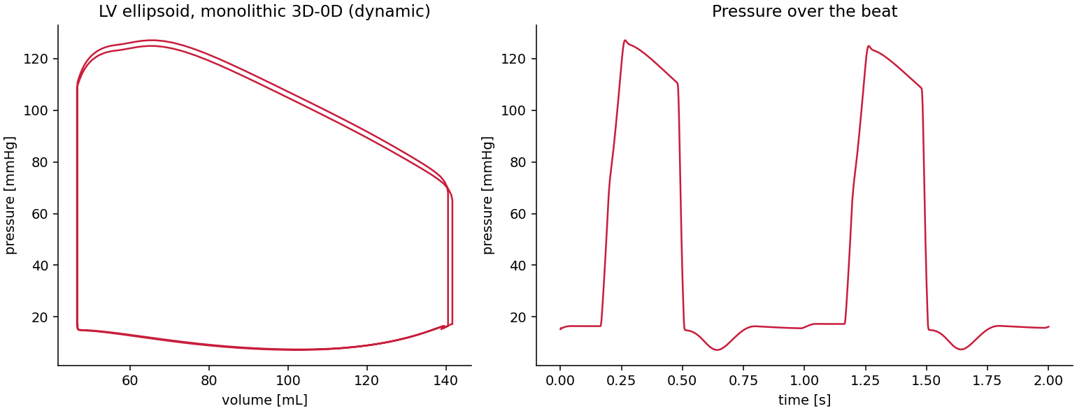
Fig. 5 Two beats of the coupled left ventricle: ejection fraction 67%, peak pressure 125 mmHg, stroke work 1.2 J. End-diastolic and end-systolic volumes move by under a percent between the two beats.#
The video shows the moving wall beside the loop it traces. The vertical limbs are the isovolumic phases, where the volume is held while the pressure runs up or down.