Crossbridges at every quadrature point in a closed-loop circulation

In this demo we put a biventricular ellipsoid into the closed-loop circulation model of Regazzoni et al. [RSA+22]. The two ventricles are the 3D model, and the atria, valves and vessels stay 0D. Contraction comes from the Land (2017) crossbridge model [LPHS+17], run at every quadrature point of the mesh and driven by a prescribed calcium transient. It is coupled to the mechanics through pulse.StabilizedActiveStress, and it is stronger in the left ventricle and the septum than in the right ventricle.

The 3D and 0D models can be coupled in three ways in these demos:

Demo	Who steps time	The 0D side is
A complete cardiac cycle on a prestressed biventricular mesh	pulse.cycle.CycleController	a phase machine with a Windkessel per ventricle
this demo	a loop in the demo	any Python function of the volumes and time
Monolithic 3D-0D coupling: an LV in a closed circulation	one Newton system	ODEs written in UFL, solved with the mechanics

Pick the split loop of this demo when the 0D model is a code you can call but not write in UFL. Here that is circulation.regazzoni2020.Regazzoni2020, whose right-hand side we evaluate once per time step.

import logging
import os
from pathlib import Path

from mpi4py import MPI

# A sibling module in this directory, not a package.
import animation
import basix
import dolfinx
import ldrb
import matplotlib.pyplot as plt
import numpy as np
import scifem
from circulation.regazzoni2020 import Regazzoni2020
from crossbridge import Land2017, calcium_trace

import cardiac_geometries
import cardiac_geometries.geometry
import pulse
from cardiac_geometries.mesh import transform_markers
from pulse.circulation import mL, mmHg

# Setup logging to print only from rank 0
class MPIFilter(logging.Filter):
    def __init__(self, comm, *args, **kwargs):
        super().__init__(*args, **kwargs)
        self.comm = comm

    def filter(self, record):
        return 1 if self.comm.rank == 0 else 0

outdir = Path("results_land_circulation_biv")
outdir.mkdir(parents=True, exist_ok=True)
geodir = outdir / "geometry"

comm = MPI.COMM_WORLD
logging.basicConfig(level=logging.INFO)
# The filter sits on the handler, so that it also catches the messages of
# other libraries' loggers.
mpi_filter = MPIFilter(comm)
for handler in logging.getLogger().handlers:
    handler.addFilter(mpi_filter)
logger = logging.getLogger("pulse")
for name in ("scifem", "matplotlib", "circulation", "ldrb"):
    logging.getLogger(name).setLevel(logging.WARNING)

We run four beats of one second each, with a time step of 1 ms. Under CI, where this page is built, the run is cut to two steps. Setting PULSE_MAX_STEPS to a positive number cuts it to that many steps instead.

_ci = os.getenv("CI", "").strip().lower()
IN_CI = _ci not in ("", "0", "false", "no", "off")
BCL = 1.0  # s, the basic cycle length
NUM_BEATS = 4
DT = 1e-3  # s
max_steps = 2 if IN_CI else int(round(NUM_BEATS * BCL / DT))
MAX_STEPS = int(os.getenv("PULSE_MAX_STEPS", "0"))
if MAX_STEPS > 0:
    max_steps = MAX_STEPS

Geometry

We use the idealized biventricular ellipsoid from cardiac-geometries, with fibres at 60° on the endocardium and -60° on the epicardium. The fibres live in a quadrature space of degree 6, the same degree we integrate with below, so the mechanics sees them exactly where it needs them.

if not (geodir / "mesh.xdmf").exists():
    logger.info("Generating the BiV ellipsoid...")
    cardiac_geometries.mesh.biv_ellipsoid(
        outdir=geodir,
        char_length=1.0,
        create_fibers=True,
        fiber_angle_epi=-60,
        fiber_angle_endo=60,
        fiber_space="Quadrature_6",
        comm=comm,
    )
comm.barrier()
geo = cardiac_geometries.geometry.Geometry.from_folder(comm=comm, folder=geodir)

INFO:pulse:Generating the BiV ellipsoid...

2026-10-10 10:42:20 [debug    ] Convert file results_land_circulation_biv/geometry/biv_ellipsoid.msh to dolfin

Info    : Reading 'results_land_circulation_biv/geometry/biv_ellipsoid.msh'...
Info    : 42 entities
Info    : 315 nodes
Info    : 1551 elements
Info    : Done reading 'results_land_circulation_biv/geometry/biv_ellipsoid.msh'

INFO:cardiac_geometries.geometry:Reading geometry from results_land_circulation_biv/geometry

Regions

To pick its fibre angles, LDRB [BBPT12] already splits a biventricular wall into left ventricle, septum and right ventricle, and returns that split as markers_scalar. We reuse it rather than drawing our own. One call with piecewise-constant (DG_0) output gives one value per cell: 1 for the LV, 2 for the RV and 3 for the septum. We turn those values into cell tags.

system = ldrb.dolfinx_ldrb(
    mesh=geo.mesh,
    ffun=geo.ffun,
    markers=transform_markers(geo.markers),
    fiber_space="DG_0",
)
system.markers_scalar.x.scatter_forward()
V0 = system.markers_scalar.function_space
cell_map = geo.mesh.topology.index_map(3)
num_cells = cell_map.size_local + cell_map.num_ghosts
cells = np.arange(num_cells, dtype=np.int32)
region_of_cell = np.rint(
    system.markers_scalar.x.array[V0.dofmap.list[cells, 0]],
).astype(np.int32)
regions = dolfinx.mesh.meshtags(geo.mesh, 3, cells, region_of_cell)
LV, RV, SEPTUM = 1, 2, 3  # ldrb's markers_scalar values
REGION_NAMES = {LV: "LV", SEPTUM: "SEPTUM", RV: "RV"}

for region, label in REGION_NAMES.items():
    count = comm.allreduce(int(np.sum(region_of_cell[: cell_map.size_local] == region)), op=MPI.SUM)
    logger.info(f"{label}: {count} cells")

INFO:pulse:LV: 337 cells

INFO:pulse:SEPTUM: 232 cells

INFO:pulse:RV: 356 cells

If pyvista is installed, we plot the three regions. The plot shows the cells of one rank only, so we skip it in parallel runs.

try:
    import pyvista
except ImportError:
    logger.info("pyvista is not installed, so we do not plot the regions")
else:
    if comm.size == 1:
        grid = pyvista.UnstructuredGrid(*dolfinx.plot.vtk_mesh(geo.mesh, 3))
        grid.cell_data["region"] = regions.values[: cell_map.size_local]
        plotter = pyvista.Plotter()
        plotter.add_mesh(
            grid,
            scalars="region",
            categories=True,
            cmap=[animation.CHAMBER_COLOURS[REGION_NAMES[r]] for r in (LV, RV, SEPTUM)],
            scalar_bar_args={"title": "1 = LV, 2 = RV, 3 = septum"},
        )
        if not pyvista.OFF_SCREEN:
            plotter.show()
        else:
            plotter.screenshot(outdir / "regions.png")

INFO:trame_server.utils.namespace:Translator(prefix=None)

INFO:wslink.backends.aiohttp:awaiting runner setup

INFO:wslink.backends.aiohttp:awaiting site startup

INFO:wslink.backends.aiohttp:Print WSLINK_READY_MSG

INFO:wslink.backends.aiohttp:Schedule auto shutdown with timeout 0

INFO:wslink.backends.aiohttp:awaiting running future

LDRB works from Laplace solutions, which do not change when the mesh is scaled, so we split the regions first and only then scale the mesh by 1.6e-2. That brings it to metres, which the cavity volume constraints assume, with cavities of a plausible size. pulse.HeartGeometry integrates with the same quadrature degree as the fibres.

geo.mesh.geometry.x[:] *= 1.6e-2
geometry = pulse.HeartGeometry.from_cardiac_geometries(geo, metadata={"quadrature_degree": 6})

A crossbridge model at every quadrature point

Ta, its stiffness Ka and the fibre stretch of the previous step all live in a quadrature space of degree 6. Each quadrature point is one cell of a vectorized Land2017 model: on every rank it holds one cell per local quadrature point, ghosts included.

Qe = basix.ufl.quadrature_element(geo.mesh.basix_cell(), value_shape=(), degree=6)
Q = dolfinx.fem.functionspace(geo.mesh, Qe)
Ta_q, Ka_q, lmbda_prev = (dolfinx.fem.Function(Q) for _ in range(3))
lmbda_prev.x.array[:] = 1.0

A cell’s quadrature points share its region. Q.dofmap.list gives the points of every cell, so we can spread the cell regions over the points. owned_q marks the points of the cells this rank owns; only those count towards the region means we record below, so no point is counted twice.

points_per_cell = Q.dofmap.list.shape[1]
num_owned = cell_map.size_local
region_q = np.empty(len(Ta_q.x.array), dtype=np.int32)
region_q[Q.dofmap.list.reshape(-1)] = np.repeat(region_of_cell, points_per_cell)
owned_q = np.zeros(len(Ta_q.x.array), dtype=bool)
owned_q[Q.dofmap.list[:num_owned].reshape(-1)] = True

Whole-organ parameters

Land et al. calibrate their model twice: once to skinned cells, which is what Land2017 uses by default, and once for whole-organ simulations. In the skinned calibration, half of the troponin binds calcium at 2.5 µM, more than twice the 1.1 µM peak of the transient we drive it with, so the muscle would barely contract here. We therefore use the whole-organ values the paper gives for the calcium sensitivity, the cooperativity and two crossbridge cycling rates.

LAND_WHOLE_ORGAN = {
    "ca50_ref": 0.805,  # uM
    "nTm": 5.0,
    "kuw": 182.0,  # 1/s
    "kws": 12.0,  # 1/s
}

A regional Tref

Tref is the reference tension of the Land model: its tension and its stiffness are both proportional to it. The whole-organ value of the paper is 120 kPa. We tuned the values by hand on this mesh instead, and use 160 kPa for the left ventricle, so that it ejects a plausible fraction of its volume. A weaker right ventricle is what keeps the pulmonary pressures low, so we give the right ventricle a smaller Tref, 90 kPa. The septum contracts with the LV by default.

As in Spatial material parameters, we build a space of simple functions on the region tags: it has one degree of freedom per tag, in the order of the tag list, so each region’s value is a single entry.

Tref = {LV: 160e3, SEPTUM: 160e3, RV: 90e3}  # Pa
S = scifem.create_space_of_simple_functions(geo.mesh, regions, [LV, SEPTUM, RV])
tref_simple = dolfinx.fem.Function(S)
tref_simple.x.array[:] = [Tref[LV], Tref[SEPTUM], Tref[RV]]

Land takes Tref in pascals, one value per cell of the model, that is per quadrature point. We get those values by interpolating the simple function into the quadrature space, and check them against each point’s region.

tref_q = dolfinx.fem.Function(Q)
tref_q.interpolate(dolfinx.fem.Expression(tref_simple, Q.element.interpolation_points))
assert np.array_equal(tref_q.x.array, np.vectorize(Tref.get)(region_q).astype(float))

cell = Land2017(
    num_cells=len(Ta_q.x.array),
    params={**LAND_WHOLE_ORGAN, "Tref": tref_q.x.array.copy()},
)
SL0 = cell.p["SL0"]  # um, the sarcomere length at zero fibre strain

Scaling Tref inside Land, rather than scaling its output afterwards, keeps Ta and Ka consistent. StabilizedActiveStress takes no scaling factor for exactly this reason: scaling Ta alone would break its stabilization.

The mechanics

The passive material is the transversely isotropic Holzapfel-Ogden model, with the compressible penalty Compressible2. The active stress is StabilizedActiveStress, which reads Ta and Ka in kilopascals, as Land returns them.

material_params = pulse.HolzapfelOgden.transversely_isotropic_parameters()
material = pulse.HolzapfelOgden(f0=geo.f0, s0=geo.s0, **material_params)
active = pulse.StabilizedActiveStress(
    geo.f0,
    activation=pulse.Variable(Ta_q, "kPa"),
    active_stiffness=pulse.Variable(Ka_q, "kPa"),
    lmbda_prev=lmbda_prev,
)
model = pulse.CardiacModel(
    material=material,
    active=active,
    compressibility=pulse.compressibility.Compressible2(),
)

A sliding base

The base may slide in its own plane but not leave it. A spring on the base is not enough: with a stiffness of 1e5 Pa/m, parts of the base rose by up to 2 cm along the long axis. Clamping the base instead would also stop it from moving inwards and outwards with the wall, which it does in a real heart. So we hold only the displacement component along the base normal at zero, as A complete cardiac cycle on a prestressed biventricular mesh does.

That condition holds a single displacement component, so we check that the base normal is the z axis, as biv_ellipsoid builds it: the base is the plane at the top of the mesh. We keep the normal to stand the mesh upright in the video.

up = animation.base_normal(geometry, "BASE")
if up[2] < 0.99:
    raise RuntimeError(
        f"the base normal is {up.round(3)}, not the z axis the sliding-base condition assumes",
    )

def sliding_base(V: dolfinx.fem.FunctionSpace) -> list[dolfinx.fem.DirichletBC]:
    facets = geometry.facet_tags.find(geometry.markers["BASE"][0])
    dofs = dolfinx.fem.locate_dofs_topological(V.sub(2), 2, facets)
    return [dolfinx.fem.dirichletbc(0.0, dofs, V.sub(2))]

The epicardium rests on a spring, as it would on the pericardium. A RobinBC spring acts along the surface normal only, so a spring on the base would push on exactly the component that the sliding base already holds at zero, and add nothing. We therefore put no spring on the base. Since the epicardium is curved, its spring also keeps the ventricles from drifting sideways in the base plane.

The spring must stay soft. It resists any growth of the two ventricles together, just as a tight pericardium does, so a stiff spring couples their filling. With 1e6 Pa/m, the left ventricle, which fills after the right one, pushed the right ventricular pressure up by more than its own. The tricuspid valve then closed, and the right ventricle stopped filling for the last half of diastole while its pressure climbed. At 5e4 Pa/m, the right ventricle almost stops filling for about 0.1 s while the left one fills, and then fills on until the next beat.

alpha_epi = pulse.Variable(
    dolfinx.fem.Constant(geometry.mesh, dolfinx.default_scalar_type(5e4)), "Pa / m",
)
robin_epi = pulse.RobinBC(value=alpha_epi, marker=geometry.markers["EPI"][0])
bcs = pulse.BoundaryConditions(robin=(robin_epi,), dirichlet=(sliding_base,))

Each cavity’s volume is prescribed by a Constant, in cubic metres, and its pressure is the Lagrange multiplier of that constraint. We start them at the volumes of the unloaded mesh. geometry.volume integrates over the facets this rank owns, so we sum it over the ranks.

lv_volume = dolfinx.fem.Constant(
    geometry.mesh, dolfinx.default_scalar_type(comm.allreduce(geometry.volume("LV"), op=MPI.SUM)),
)
rv_volume = dolfinx.fem.Constant(
    geometry.mesh, dolfinx.default_scalar_type(comm.allreduce(geometry.volume("RV"), op=MPI.SUM)),
)
logger.info(
    f"Unloaded volumes: LV={float(lv_volume.value) / mL:.2f} mL, "
    f"RV={float(rv_volume.value) / mL:.2f} mL",
)

INFO:pulse:Unloaded volumes: LV=115.86 mL, RV=66.34 mL

problem = pulse.StaticProblem(
    model=model,
    geometry=geometry,
    bcs=bcs,
    cavities=[
        pulse.problem.Cavity(marker="LV", volume=lv_volume),
        pulse.problem.Cavity(marker="RV", volume=rv_volume),
    ],
    parameters={"mesh_unit": "m", "base_bc": pulse.BaseBC.free},
)

The 3D side of the coupling

The circulation asks for the two ventricular pressures, given the two volumes and the time. p_BiV answers by following the protocol in the docstring of StabilizedActiveStress:

1. advance Land over one step, from \(t\) to \(t + \Delta t\), with the calcium concentration of time \(t\) and the sarcomere lengths \(SL = SL_0 \lambda_{prev}\), where \(\lambda_{prev}\) is the fibre stretch that update_prev stored after the previous solve;

2. write Land’s tension and stiffness into Ta and Ka;

3. prescribe the two volumes and solve;

4. store the new fibre stretch with update_prev.

The active stress the mechanics sees is \(T_a + K_a(\lambda - \lambda_{prev})\) along the fibres. The second term is what makes this staggered scheme work. Without it, Regazzoni and Quarteroni [RQ21] show that Ta and λ oscillate as soon as the active stiffness exceeds the passive one, which is routine in contracting muscle. The scheme is then not even convergent, and a smaller time step makes it worse.

problem.solve() returns False if Newton fails. We check it: carrying on would hand the circulation the pressures of a failed solve, and store a stretch that Land would contract from at the next step. Instead we put the problem back to its state before the solve and stop.

The calcium transient, crossbridge.calcium_trace, repeats every BCL and starts 0.1 s into each beat. That is also when the default 0D ventricles of Regazzoni2020, which the 3D model replaces, start to contract.

state = {"p_LV": 0.0, "p_RV": 0.0}

def advance_land(t: float) -> None:
    SL = SL0 * lmbda_prev.x.array
    Ca = float(calcium_trace(np.array([t % BCL]))[0])  # uM
    cell.advance_step(DT, Ca, SL)
    Ta_q.x.array[:] = cell.get_active_tension()  # kPa
    Ka_q.x.array[:] = cell.get_active_stiffness()  # kPa
    # A ghost point repeats a point another rank owns; take the owner's value.
    Ta_q.x.scatter_forward()
    Ka_q.x.scatter_forward()

def p_BiV(V_LV: float, V_RV: float, t: float) -> tuple[float, float]:
    advance_land(t)
    lv_volume.value = V_LV * mL
    rv_volume.value = V_RV * mL
    if not problem.solve():
        problem.reset_states()
        raise RuntimeError(
            f"3D solve failed at t={t:.4f} s (V_LV={V_LV:.2f} mL, V_RV={V_RV:.2f} mL)",
        )
    active.update_prev(problem.u)
    lmbda_prev.x.scatter_forward()
    state["p_LV"] = float(problem.cavity_pressures[0].x.array[0]) / mmHg
    state["p_RV"] = float(problem.cavity_pressures[1].x.array[0]) / mmHg
    return state["p_LV"], state["p_RV"]

The 0D side and the loop

Regazzoni2020 calls p_BiV for the ventricular pressures, and its own time-varying elastances for the atria. We set its heart rate to 1 / BCL, so the atria beat with the same period as the calcium transient. They contract 0.9 s into each beat, shortly before the next transient starts.

Less blood than the defaults

The default initial state of Regazzoni2020 suits its own 0D ventricles, not this mesh. Its right ventricle holds 166 mL at a pressure of a few mmHg; the 3D right ventricle is much stiffer, and is unloaded at 66 mL. With the default blood volume, the blood the ventricles cannot take backs up into the atria and veins, and the filling pressures climb well above normal. So the two ventricular volumes start at the unloaded volumes of the mesh, and the atria, the veins and the pulmonary arteries start at 60% of their default volumes and pressures. All other states keep their defaults. That leaves 1030 mL in the circuit, 588 mL less than the defaults. Even so, the first beats move blood between the compartments until the closed loop settles; this is why we run four beats and judge the last.

Regazzoni2020 has its own solve, but we do not use it: the loop below is the whole time stepping. Building the model does not call p_BiV, so Land is first advanced inside the loop. Each step evaluates the right-hand side once at the start of the step. That makes exactly one call to p_BiV, and so one 3D solve, at the volumes \(V_n\) and the time \(t_n\). A forward Euler step then advances the twelve circuit states. The 3D model only ever sees volumes that are known, so the coupling needs no iteration between the two models.

The circuit’s elastances repeat every beat on their own, so we pass them the global time, as we do for the calcium transient.

FILL = 0.6  # the fraction of the default atrial volumes and vessel pressures we keep
defaults = {k: v.magnitude for k, v in Regazzoni2020.default_initial_conditions().items()}
initial_state = {
    **defaults,  # mL, mmHg and mL/s
    "V_LV": float(lv_volume.value) / mL,
    "V_RV": float(rv_volume.value) / mL,
    **{k: FILL * defaults[k] for k in ("V_LA", "V_RA", "p_VEN_SYS", "p_VEN_PUL", "p_AR_PUL")},
}
circ = Regazzoni2020(
    add_units=False,
    p_BiV=p_BiV,
    parameters={"HR": 1.0 / BCL},
    initial_state=initial_state,
    outdir=outdir,
    comm=comm,
)
names = list(circ.state_names())

The volume the circuit holds is that of the four chambers plus, for each vessel, its compliance times its pressure. The circuit conserves it, so we can compare the two initial states by it.

def circuit_volume(states: dict[str, float]) -> float:
    vessels = circ.parameters["circulation"]
    return sum(states[f"V_{c}"] for c in ("LA", "LV", "RA", "RV")) + sum(
        vessels[side]["C_AR"] * states[f"p_AR_{side}"] + vessels[side]["C_VEN"] * states[f"p_VEN_{side}"]
        for side in ("SYS", "PUL")
    )

logger.info(
    f"The circuit holds {circuit_volume(initial_state):.0f} mL, "
    f"{circuit_volume(defaults) - circuit_volume(initial_state):.0f} mL less than with the defaults",
)
y = np.asarray(circ.state, dtype=float).copy()

INFO:pulse:The circuit holds 1030 mL, 588 mL less than with the defaults

At each step we record the states \(y_n\) together with the pressures computed from them, so a recorded pressure and volume always belong together. Ta and the sarcomere length are averaged over each region. We also keep the moving geometry every ten steps, so that make_animations.py can render it afterwards. FrameRecorder keeps each rank’s part of the mesh separately, so we only record frames in serial runs, and never under CI.

def region_mean(values: np.ndarray, region: int) -> float:
    mask = owned_q & (region_q == region)
    total = comm.allreduce(float(values[mask].sum()), op=MPI.SUM)
    count = comm.allreduce(int(mask.sum()), op=MPI.SUM)
    return total / count

history: dict[str, list[float]] = {
    k: []
    for k in (
        "time", "p_LV", "p_RV", "Ta_LV", "Ta_SEPTUM", "Ta_RV", "SL_LV", "SL_SEPTUM", "SL_RV",
        *names,
    )
}
recorder = animation.FrameRecorder(
    geometry.mesh, every=10, enabled=not IN_CI and comm.size == 1, up=up,
)
vtx = dolfinx.io.VTXWriter(comm, outdir / "displacement.bp", [problem.u], engine="BP4")

logger.info(f"Running {max_steps} steps of {DT * 1e3:.0f} ms...")
for n in range(max_steps):
    t = n * DT
    dy = circ.rhs(t, y)  # one 3D solve at (V_n, t_n); p_BiV stashes its pressures
    history["time"].append(t)
    history["p_LV"].append(state["p_LV"])
    history["p_RV"].append(state["p_RV"])
    for i, name in enumerate(names):
        history[name].append(y[i])  # y_n, the states the pressures came from
    for region, label in REGION_NAMES.items():
        history[f"Ta_{label}"].append(region_mean(Ta_q.x.array, region))
        history[f"SL_{label}"].append(region_mean(SL0 * lmbda_prev.x.array, region))
    recorder.record(problem.u, t, n)
    if n % 10 == 0:
        vtx.write(t)
    if n % 10 == 0 or n == max_steps - 1:
        logger.info(
            f"t={t:.3f} s: p_LV={state['p_LV']:.4f} mmHg, p_RV={state['p_RV']:.4f} mmHg, "
            f"V_LV={y[names.index('V_LV')]:.3f} mL, V_RV={y[names.index('V_RV')]:.3f} mL, "
            f"Ta_LV={history['Ta_LV'][-1]:.3f} kPa",
        )
    y = y + DT * dy  # forward Euler on the circuit
vtx.close()
logger.info("Simulation complete.")

INFO:pulse:Running 2 steps of 1 ms...

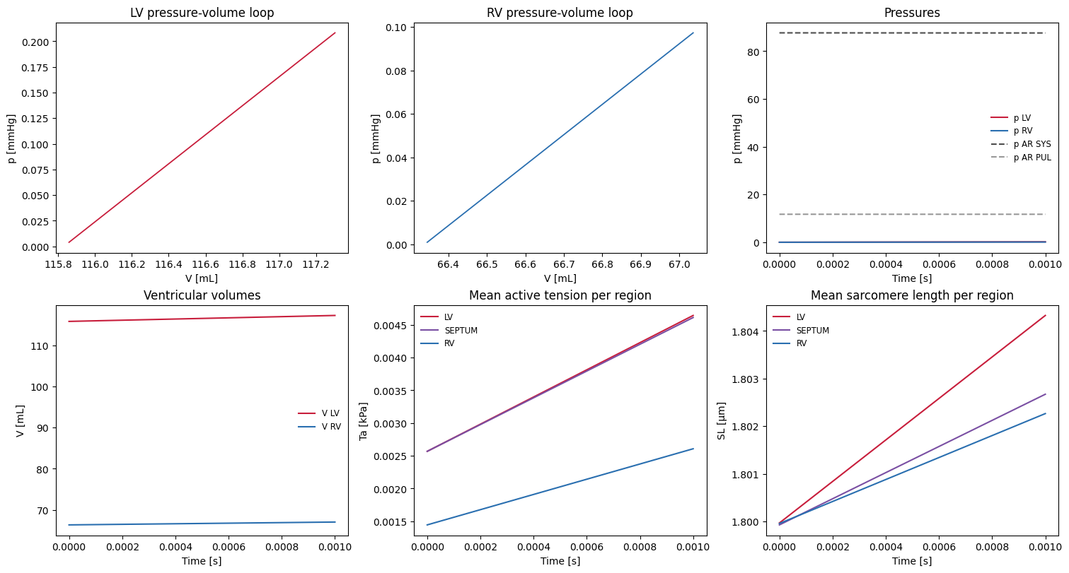
INFO:pulse:t=0.000 s: p_LV=0.0040 mmHg, p_RV=0.0009 mmHg, V_LV=115.859 mL, V_RV=66.345 mL, Ta_LV=0.003 kPa

INFO:pulse:t=0.001 s: p_LV=0.2083 mmHg, p_RV=0.0973 mmHg, V_LV=117.303 mL, V_RV=67.036 mL, Ta_LV=0.005 kPa

INFO:pulse:Simulation complete.

Results

We save the traces (volumes in mL, pressures in mmHg, flows in mL/s, Ta in kPa and sarcomere lengths in µm) and the recorded frames, and plot them.

if comm.rank == 0:
    traces = {k: np.asarray(v) for k, v in history.items()}
    np.savez(outdir / "traces.npz", **traces)
saved = recorder.save(outdir / "frames.npz")
if saved is not None:
    logger.info(f"Saved {len(recorder.times)} frames of the moving geometry to {saved}")

if comm.rank == 0:
    fig, axes = plt.subplots(2, 3, figsize=(15, 8), layout="constrained")
    for ax_loop, name in zip(axes[0, :2], ("LV", "RV")):
        ax_loop.plot(
            traces[f"V_{name}"], traces[f"p_{name}"],
            color=animation.CHAMBER_COLOURS[name], linewidth=1.3,
        )
        ax_loop.set_xlabel("V [mL]")
        ax_loop.set_ylabel("p [mmHg]")
        ax_loop.set_title(f"{name} pressure-volume loop")
    ax_p, ax_v, ax_ta, ax_sl = axes[0, 2], axes[1, 0], axes[1, 1], axes[1, 2]
    for name in ("LV", "RV"):
        colour = animation.CHAMBER_COLOURS[name]
        ax_p.plot(traces["time"], traces[f"p_{name}"], color=colour, label=f"p {name}")
        ax_v.plot(traces["time"], traces[f"V_{name}"], color=colour, label=f"V {name}")
    ax_p.plot(traces["time"], traces["p_AR_SYS"], color="0.3", linestyle="--", label="p AR SYS")
    ax_p.plot(traces["time"], traces["p_AR_PUL"], color="0.6", linestyle="--", label="p AR PUL")
    for label in REGION_NAMES.values():
        colour = animation.CHAMBER_COLOURS[label]
        ax_ta.plot(traces["time"], traces[f"Ta_{label}"], color=colour, label=label)
        ax_sl.plot(traces["time"], traces[f"SL_{label}"], color=colour, label=label)
    for axis, ylabel, title in (
        (ax_p, "p [mmHg]", "Pressures"),
        (ax_v, "V [mL]", "Ventricular volumes"),
        (ax_ta, "Ta [kPa]", "Mean active tension per region"),
        (ax_sl, "SL [µm]", "Mean sarcomere length per region"),
    ):
        axis.set_xlabel("Time [s]")
        axis.set_ylabel(ylabel)
        axis.set_title(title)
        axis.legend(frameon=False, fontsize="small")
    fig.savefig(outdir / "land_circulation_biv.png", dpi=140)
    plt.show()

    if not IN_CI:
        # The end-diastolic and end-systolic volumes are the largest and the
        # smallest volume of the last complete beat. A run shorter than one
        # beat reports the beat it is in.
        time = traces["time"]
        complete = int(np.floor((time[-1] + DT) / BCL + 1e-9))
        beat = max(complete - 1, 0)
        in_beat = (time >= beat * BCL - 1e-9) & (time < (beat + 1) * BCL - 1e-9)
        label = f"beat {beat + 1}" + ("" if complete > 0 else " (incomplete)")
        for name in ("LV", "RV"):
            V_beat = traces[f"V_{name}"][in_beat]
            EDV, ESV = float(V_beat.max()), float(V_beat.min())
            peak = float(traces[f"p_{name}"][in_beat].max())
            logger.info(
                f"{name}, {label}: EDV {EDV:.1f} mL, ESV {ESV:.1f} mL, SV {EDV - ESV:.1f} mL, "
                f"EF {100 * (1 - ESV / EDV):.1f}%, peak {peak:.1f} mmHg",
            )

A whole beat

The figure and the video come from a full run kept in _static/, rather than from the two steps this page takes under CI. To regenerate them, run

python3 land_circulation_biv.py
python3 make_animations.py land_circulation_biv

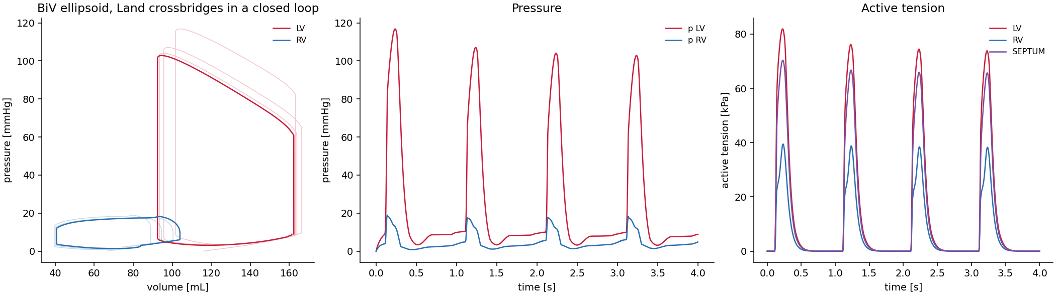
Fig. 2 Both ventricles over four beats, the last one drawn solid and the earlier ones faded. In the last beat the left ventricle ejects 70 mL (EF 43%) against a peak of 103 mmHg, and the right 63 mL (EF 61%) against 18 mmHg. Just before the calcium transient starts, the left ventricular pressure is 10 mmHg and the right 6 mmHg. The earlier beats drift while the closed loop settles from its initial state: the left ventricular peak falls from 117 to 103 mmHg, and the right ventricular end-diastolic volume grows from 89 to 104 mL. In the last beat both loops close to within about 2 mL.

Frank–Starling for free

Land’s model makes tension depend on sarcomere length: beta0 raises the maximal tension and beta1 the calcium sensitivity as the sarcomere lengthens. A ventricle that fills more therefore contracts harder, without any extra code. Isometric Twitch with the Land (2017) Cross-Bridge Model shows the same effect in an isometric twitch.

References

[BBPT12]

Jason D Bayer, Robert C Blake, Gernot Plank, and Natalia A Trayanova. A novel rule-based algorithm for assigning myocardial fiber orientation to computational heart models. Annals of Biomedical Engineering, 40(10):2243–2254, 2012. doi:10.1007/s10439-012-0593-5.

[LPHS+17]

Sander Land, So-Jin Park-Holohan, Nicolas P Smith, Cristobal G Dos Remedios, Jonathan C Kentish, and Steven A Niederer. A model of cardiac contraction based on novel measurements of tension development in human cardiomyocytes. Journal of molecular and cellular cardiology, 106:68–83, 2017. doi:10.1016/j.yjmcc.2017.03.008.

[RQ21]

Francesco Regazzoni and Alfio Quarteroni. An oscillation-free fully staggered algorithm for velocity-dependent active models of cardiac mechanics. Computer Methods in Applied Mechanics and Engineering, 373:113506, 2021. doi:10.1016/j.cma.2020.113506.

[RSA+22]

Francesco Regazzoni, Matteo Salvador, Pasquale Claudio Africa, Marco Fedele, Luca Dedè, and Alfio Quarteroni. A cardiac electromechanical model coupled with a lumped-parameter model for closed-loop blood circulation. Journal of Computational Physics, 457:111083, 2022. doi:10.1016/j.jcp.2022.111083.