Isometric Twitch with the Lewalle (2024) OFF-State Feedback Model

This demo repeats the Land (2017) cross-bridge twitch with crossbridge’s Lewalle2024 model instead. Lewalle2024 is Land (2017) with one deliberate change: the two ad hoc length-dependent-activation gradients beta0 (shifts peak tension with sarcomere length) and beta1 (shifts calcium sensitivity with sarcomere length) are switched off (beta0 = beta1 = 0 in its default parameters) and replaced with an explicit mechanism – myosin thick-filament OFF-state force feedback [LMCN24].

What “OFF-state feedback” means physically

Land (2017) treats every myosin head as available to cycle (unbound/pre-/post-powerstroke); Lewalle (2024) adds a fourth, force-recruited possibility – an OFF state in which the head is sequestered against the thick filament backbone and cannot bind actin at all. Two extra populations, BE and UE, mirror B and U but with the head OFF; transition rates k1/k2 between ON and OFF depend on the tissue’s own force output (params["which_dep"], default "totalforce"), so more force recruits more heads OFF the backbone. This is a feedback loop: cross-bridges generate force, force pulls more heads OFF, which throttles further force generation. Because that feedback is itself length-sensitive (a longer sarcomere reaches a given force at a lower fraction of attached heads), it reproduces length-dependent activation without curve-fitting it directly – the Frank-Starling effect falls out of thick-filament mechanics instead of two tuned constants.

Calcium scale

Lewalle2024’s default calcium sensitivity (pCa50ref = 5.25, i.e. \(\mathrm{Ca}_{50} \approx 5.6\,\mu M\)) is calibrated against skinned-fiber experiments, which use much higher free calcium than an intact myocyte’s transient. crossbridge.calcium_trace’s own default peak (1.1 \(\mu\)M, tuned for intact-cell-scale transients) therefore drives this particular calibration only slightly above baseline. We raise the peak to 6 \(\mu\)M here (calcium_trace(..., cmax=6.0)) purely so the twitch is clearly visible – see the comparison demo for a discussion of how much this scale varies model-to-model.

The pulse coupling is identical to the Land (2017) demo: Lewalle2024 exposes the same get_active_tension()/get_active_stiffness() interface, consumed by pulse.StabilizedActiveStress.

from mpi4py import MPI

import dolfinx
import matplotlib.pyplot as plt
import numpy as np
import ufl
from crossbridge import Lewalle2024, calcium_trace

import pulse

1. The isometric twitch experiment

CA_CMAX = 6.0  # uM -- see markdown above for why this differs from the package default


def run_isometric_twitch(pre_stretch_mm: float, t_end: float = 0.6, couple_dt: float = 1e-2):
    """
    Runs an isometric twitch on a 10x1x1 mm slab, driven by the Lewalle
    (2024) OFF-state feedback cross-bridge model.

    Returns the passive fiber stress, and (time, active fiber stress) arrays.
    """
    L = 10.0
    mesh = dolfinx.mesh.create_box(
        MPI.COMM_WORLD,
        [[0.0, 0.0, 0.0], [L, 1.0, 1.0]],
        [10, 2, 2],
    )

    f0 = dolfinx.fem.Constant(mesh, dolfinx.default_scalar_type((1.0, 0.0, 0.0)))
    s0 = dolfinx.fem.Constant(mesh, dolfinx.default_scalar_type((0.0, 1.0, 0.0)))

    Ta = pulse.Variable(dolfinx.fem.Constant(mesh, dolfinx.default_scalar_type(0.0)), "kPa")
    Ka = pulse.Variable(dolfinx.fem.Constant(mesh, dolfinx.default_scalar_type(0.0)), "kPa")

    material_params = pulse.HolzapfelOgden.transversely_isotropic_parameters()
    passive_model = pulse.HolzapfelOgden(f0=f0, s0=s0, **material_params)
    active_model = pulse.StabilizedActiveStress(f0=f0, activation=Ta, active_stiffness=Ka)

    model = pulse.CardiacModel(
        material=passive_model,
        active=active_model,
        compressibility=pulse.Compressible2(),
    )

    boundaries = [
        pulse.Marker(name="X0", marker=1, dim=2, locator=lambda x: np.isclose(x[0], 0)),
        pulse.Marker(name="X1", marker=2, dim=2, locator=lambda x: np.isclose(x[0], L)),
    ]
    geo = pulse.Geometry(mesh=mesh, boundaries=boundaries, metadata={"quadrature_degree": 4})

    def dirichlet_bc(V: dolfinx.fem.FunctionSpace) -> list[dolfinx.fem.bcs.DirichletBC]:
        mesh.topology.create_connectivity(mesh.topology.dim - 1, mesh.topology.dim)

        facets_fixed = geo.facet_tags.find(1)
        dofs = dolfinx.fem.locate_dofs_topological(V, 2, facets_fixed)
        u_fixed = dolfinx.fem.Function(V)
        u_fixed.x.array[:] = 0.0

        facets_stretch = geo.facet_tags.find(2)
        V_x, _ = V.sub(0).collapse()
        dofs_x = dolfinx.fem.locate_dofs_topological((V.sub(0), V_x), 2, facets_stretch)
        u_stretch_x = dolfinx.fem.Function(V_x)
        u_stretch_x.x.array[:] = pre_stretch_mm

        return [
            dolfinx.fem.dirichletbc(u_stretch_x, dofs_x, V.sub(0)),
            dolfinx.fem.dirichletbc(u_fixed, dofs),
        ]

    bcs = pulse.BoundaryConditions(dirichlet=(dirichlet_bc,))
    parameters = {"mesh_unit": "mm"}
    problem = pulse.StaticProblem(model=model, geometry=geo, bcs=bcs, parameters=parameters)

    Vs = dolfinx.fem.functionspace(mesh, ("DG", 1))
    active_model.lmbda_prev = dolfinx.fem.Function(Vs)
    active_model.lmbda_prev.x.array[:] = 1.0

    # --- Phase 1: passive pre-stretch ---
    problem.solve()

    F = ufl.variable(ufl.grad(problem.u) + ufl.Identity(3))
    f = F * f0
    f_norm = f / ufl.sqrt(ufl.inner(f, f))
    volume = mesh.comm.allreduce(
        dolfinx.fem.assemble_scalar(dolfinx.fem.form(ufl.det(F) * geo.dx)),
        op=MPI.SUM,
    )
    Tf = dolfinx.fem.form(ufl.inner(model.sigma(F) * f_norm, f_norm) * geo.dx)
    passive_force = mesh.comm.allreduce(dolfinx.fem.assemble_scalar(Tf), op=MPI.SUM) / volume

    # --- Phase 2: standalone cross-bridge twitch at the fixed sarcomere length ---
    cell = Lewalle2024(num_cells=1)
    SL0 = cell.p["SL0"]
    lmbda_pre = 1.0 + pre_stretch_mm / L
    SL_fixed = SL0 * lmbda_pre

    dt_cell = cell.dt
    couple_every = max(1, round(couple_dt / dt_cell))
    n_steps = int(round(t_end / dt_cell))

    times, active_stresses = [], []
    t = 0.0
    for i in range(n_steps):
        Ca = calcium_trace(np.array([t]), cmax=CA_CMAX)[0]
        cell.advance_step(dt_cell, Ca, SL_fixed)
        t += dt_cell

        if i % couple_every == 0:
            Ta.assign(float(cell.get_active_tension()[0]))
            Ka.assign(float(cell.get_active_stiffness()[0]))
            problem.solve()
            active_model.update_prev(problem.u)

            total_force = mesh.comm.allreduce(dolfinx.fem.assemble_scalar(Tf), op=MPI.SUM) / volume
            times.append(t)
            active_stresses.append(total_force - passive_force)

    return passive_force, np.array(times), np.array(active_stresses)

2. Running twitches at increasing pre-stretch

stretch_amounts = [0.0, 0.5, 1.0, 1.5]  # mm, i.e. 0%, 5%, 10%, 15% strain
strain_pcts = [(s / 10.0) * 100 for s in stretch_amounts]

passive_stresses = []
traces = []

for s, pct in zip(stretch_amounts, strain_pcts):
    p_force, times, active = run_isometric_twitch(s)
    passive_stresses.append(p_force)
    traces.append((times, active))
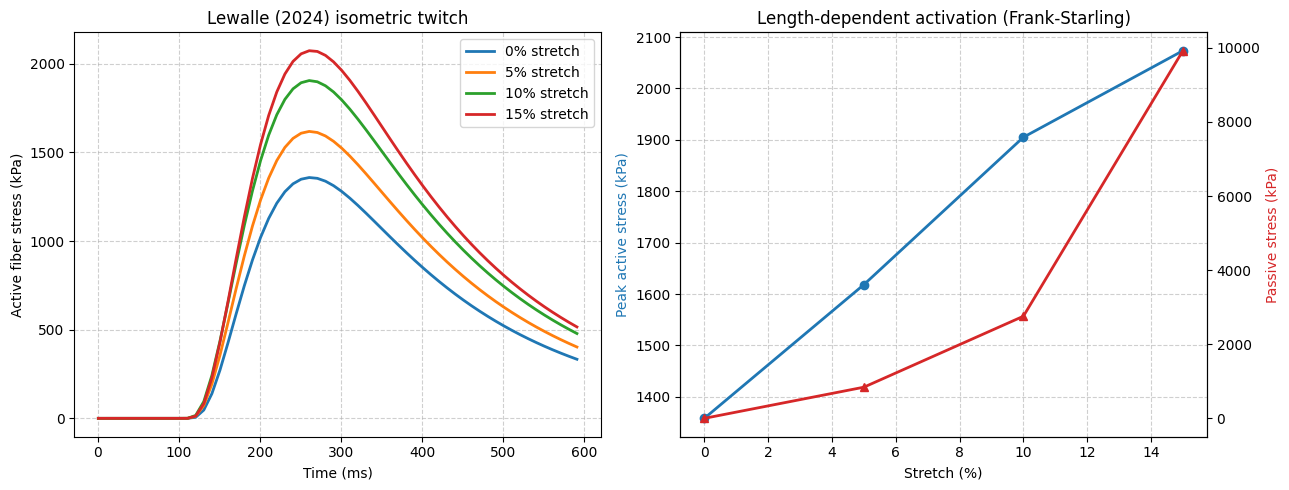
    print(f"stretch {pct:5.1f}%  passive={p_force:8.4f} kPa  peak active={active.max():8.4f} kPa")

stretch   0.0%  passive=  0.0000 kPa  peak active=905.4718 kPa

stretch   5.0%  passive=840.7423 kPa  peak active=1103.9165 kPa

stretch  10.0%  passive=2755.5774 kPa  peak active=1292.1579 kPa

stretch  15.0%  passive=9921.8714 kPa  peak active=1220.3673 kPa

3. Plotting the results

fig, (ax1, ax2) = plt.subplots(1, 2, figsize=(13, 5))

for (times, active), pct in zip(traces, strain_pcts):
    ax1.plot(times * 1000, active, linewidth=2, label=f"{pct:.0f}% stretch")
ax1.set_xlabel("Time (ms)")
ax1.set_ylabel("Active fiber stress (kPa)")
ax1.set_title("Lewalle (2024) isometric twitch")
ax1.legend()
ax1.grid(True, linestyle="--", alpha=0.6)

peak_active = [active.max() for _, active in traces]
ax2.plot(
    strain_pcts, peak_active, marker="o", linewidth=2, color="tab:blue", label="Peak active stress",
)
ax2b = ax2.twinx()
ax2b.plot(
    strain_pcts, passive_stresses, marker="^", linewidth=2, color="tab:red", label="Passive stress",
)
ax2.set_xlabel("Stretch (%)")
ax2.set_ylabel("Peak active stress (kPa)", color="tab:blue")
ax2b.set_ylabel("Passive stress (kPa)", color="tab:red")
ax2.set_title("Length-dependent activation (Frank-Starling)")
ax2.grid(True, linestyle="--", alpha=0.6)

fig.tight_layout()
plt.show()

4. Conclusion

Lewalle2024 reproduces the ascending limb of the Frank-Starling curve seen with Land2017 at moderate pre-stretch, but by a different route: instead of two length-dependence gradients tuned directly against force-length data, the effect emerges from a force-feedback loop on myosin’s ON/OFF equilibrium.

That same feedback also explains why peak active stress drops again at the largest pre-stretch tested here (15%): which_dep="totalforce" (the default) recruits myosin heads OFF the thick filament in proportion to total fiber stress, active and passive combined. At 15% pre-stretch the passive Holzapfel-Ogden matrix alone is already generating ~10x the stress it does at 10%, and that passive load is enough to throttle cycling through the same feedback that produces the ascending limb at lower stretch. This is a genuine consequence of coupling force feedback (as opposed to Land2017’s length-only gradients) to a strongly nonlinear passive material, not an artifact – see params["which_dep"] in Lewalle2024.default_parameters() for the other feedback variants the package supports ("force" restricts the feedback to the active contribution alone, "passiveforce" to the passive one, "Lambda" drops force-dependence entirely).

Whether this differs in shape (rise time, relaxation) from Land2017 at the stretch levels where both curves ascend is exactly what the comparison demo checks.

References

[LMCN24]

Alexandre Lewalle, Gregory Milburn, Kenneth S Campbell, and Steven A Niederer. Cardiac length-dependent activation driven by force-dependent thick-filament dynamics. Biophysical Journal, 123(18):2996–3009, 2024. doi:10.1016/j.bpj.2024.05.025.