
Isometric Twitch with the Land (2017) Cross-Bridge Model#
The frank_starling_twitch demo reproduces the
Frank-Starling mechanism with a purely phenomenological, curve-fitted
multiplier \(g(\lambda)\) bolted onto the active stress. This demo replaces
that ad hoc multiplier with a genuine sub-cellular force-generation model:
crossbridge’s
implementation of the Land et al. model [LPHS+17].
Why a cross-bridge model instead of a fitted curve#
The Land model integrates troponin-C calcium binding (CaTRPN) into a
three-state thick/thin-filament cycle – unbound (U), pre-powerstroke
(W), post-powerstroke (S) – with a distortion-decay description of
cross-bridge strain. Active tension is a direct readout of that state, so
feeding it a realistic intracellular calcium transient reproduces an actual
twitch: a rise, a peak, and a relaxation, rather than a single
steady-state activation level. Length dependence enters through two
empirical gradients, beta0 (shifts peak tension with sarcomere length)
and beta1 (shifts calcium sensitivity, i.e. \(\mathrm{pCa}_{50}\), with
sarcomere length) – still curve-fitted, but now acting on a mechanistic
cross-bridge population instead of standing in for the whole active
stress.
Coupling to pulse#
crossbridge models expose exactly the two quantities
pulse.StabilizedActiveStress needs from an external
force-generation model: get_active_tension() (\(T_a\)) and
get_active_stiffness() (\(K_a = \partial\dot T_a/\partial\dot\lambda\)).
Using the stabilized formulation – rather than plain
pulse.ActiveStress – is the documented way to consume such a
model; see its docstring, and [RQ21], for why a
naive staggered coupling can be unstable once active stiffness exceeds
passive stiffness.
crossbridge works in sarcomere length (SL, in \(\mu\)m), while pulse
works in fiber stretch \(\lambda\) (dimensionless, relative to the FEM
reference configuration). We map between them with
\(\mathrm{SL}(\lambda) = \mathrm{SL}_0 \cdot \lambda\), taking each model’s
own resting sarcomere length SL0 as the length corresponding to the
undeformed geometry. This is a modeling choice made here for the demo, not
something either package infers automatically.
Since the tissue is held isometric (both end faces have prescribed displacement), \(\lambda\) does not evolve during the twitch – only \(T_a(t)\) does – so we drive the cell model standalone over the calcium transient and only invoke the FEM solve at a handful of coupling points along that trace.
from mpi4py import MPI

import dolfinx
import matplotlib.pyplot as plt
import numpy as np
import ufl
from crossbridge import Land2017, calcium_trace

import pulse
1. The isometric twitch experiment#
As in the original demo we use a 10x1x1 mm slab with fibers along \(x\),
stretch the right face by a prescribed amount and lock both faces
(isometric condition), then activate. Here activation comes from
standalone-integrating Land2017 over a calcium transient at the fixed
sarcomere length implied by the pre-stretch, and feeding its \(T_a(t)\),
\(K_a(t)\) into pulse.StabilizedActiveStress at each coupling point.
def run_isometric_twitch(pre_stretch_mm: float, t_end: float = 0.6, couple_dt: float = 1e-2):
    """
    Runs an isometric twitch on a 10x1x1 mm slab, driven by the Land (2017)
    cross-bridge model.

    1. Stretches the right face by `pre_stretch_mm` and locks it.
    2. Integrates `Land2017` over a calcium transient at the resulting fixed
       sarcomere length.
    3. Drives the mechanics problem through that twitch via
       `StabilizedActiveStress`, sampled every `couple_dt` seconds.

    Returns the passive fiber stress, and (time, active fiber stress) arrays.
    """
    L = 10.0
    mesh = dolfinx.mesh.create_box(
        MPI.COMM_WORLD,
        [[0.0, 0.0, 0.0], [L, 1.0, 1.0]],
        [10, 2, 2],
    )

    f0 = dolfinx.fem.Constant(mesh, dolfinx.default_scalar_type((1.0, 0.0, 0.0)))
    s0 = dolfinx.fem.Constant(mesh, dolfinx.default_scalar_type((0.0, 1.0, 0.0)))

    Ta = pulse.Variable(dolfinx.fem.Constant(mesh, dolfinx.default_scalar_type(0.0)), "kPa")
    Ka = pulse.Variable(dolfinx.fem.Constant(mesh, dolfinx.default_scalar_type(0.0)), "kPa")

    material_params = pulse.HolzapfelOgden.transversely_isotropic_parameters()
    passive_model = pulse.HolzapfelOgden(f0=f0, s0=s0, **material_params)
    active_model = pulse.StabilizedActiveStress(f0=f0, activation=Ta, active_stiffness=Ka)

    model = pulse.CardiacModel(
        material=passive_model,
        active=active_model,
        compressibility=pulse.Compressible2(),
    )

    boundaries = [
        pulse.Marker(name="X0", marker=1, dim=2, locator=lambda x: np.isclose(x[0], 0)),
        pulse.Marker(name="X1", marker=2, dim=2, locator=lambda x: np.isclose(x[0], L)),
    ]
    geo = pulse.Geometry(mesh=mesh, boundaries=boundaries, metadata={"quadrature_degree": 4})

    def dirichlet_bc(V: dolfinx.fem.FunctionSpace) -> list[dolfinx.fem.bcs.DirichletBC]:
        mesh.topology.create_connectivity(mesh.topology.dim - 1, mesh.topology.dim)

        facets_fixed = geo.facet_tags.find(1)
        dofs = dolfinx.fem.locate_dofs_topological(V, 2, facets_fixed)
        u_fixed = dolfinx.fem.Function(V)
        u_fixed.x.array[:] = 0.0

        facets_stretch = geo.facet_tags.find(2)
        V_x, _ = V.sub(0).collapse()
        dofs_x = dolfinx.fem.locate_dofs_topological((V.sub(0), V_x), 2, facets_stretch)
        u_stretch_x = dolfinx.fem.Function(V_x)
        u_stretch_x.x.array[:] = pre_stretch_mm

        return [
            dolfinx.fem.dirichletbc(u_stretch_x, dofs_x, V.sub(0)),
            dolfinx.fem.dirichletbc(u_fixed, dofs),
        ]

    bcs = pulse.BoundaryConditions(dirichlet=(dirichlet_bc,))
    parameters = {"mesh_unit": "mm"}
    problem = pulse.StaticProblem(model=model, geometry=geo, bcs=bcs, parameters=parameters)

    # lmbda_prev must be a Function (not a Constant) to track the (spatially
    # near-uniform) fiber stretch between coupling points, per
    # StabilizedActiveStress.update_prev.
    Vs = dolfinx.fem.functionspace(mesh, ("DG", 1))
    active_model.lmbda_prev = dolfinx.fem.Function(Vs)
    active_model.lmbda_prev.x.array[:] = 1.0

    # --- Phase 1: passive pre-stretch ---
    problem.solve()

    F = ufl.variable(ufl.grad(problem.u) + ufl.Identity(3))
    f = F * f0
    f_norm = f / ufl.sqrt(ufl.inner(f, f))
    volume = mesh.comm.allreduce(
        dolfinx.fem.assemble_scalar(dolfinx.fem.form(ufl.det(F) * geo.dx)),
        op=MPI.SUM,
    )
    Tf = dolfinx.fem.form(ufl.inner(model.sigma(F) * f_norm, f_norm) * geo.dx)
    passive_force = mesh.comm.allreduce(dolfinx.fem.assemble_scalar(Tf), op=MPI.SUM) / volume

    # --- Phase 2: standalone cross-bridge twitch at the fixed sarcomere length ---
    cell = Land2017(num_cells=1)
    SL0 = cell.p["SL0"]
    lmbda_pre = 1.0 + pre_stretch_mm / L
    SL_fixed = SL0 * lmbda_pre

    dt_cell = cell.dt
    couple_every = max(1, round(couple_dt / dt_cell))
    n_steps = int(round(t_end / dt_cell))

    times, active_stresses = [], []
    t = 0.0
    for i in range(n_steps):
        Ca = calcium_trace(np.array([t]))[0]
        cell.advance_step(dt_cell, Ca, SL_fixed)
        t += dt_cell

        if i % couple_every == 0:
            Ta.assign(float(cell.get_active_tension()[0]))
            Ka.assign(float(cell.get_active_stiffness()[0]))
            problem.solve()
            active_model.update_prev(problem.u)

            total_force = mesh.comm.allreduce(dolfinx.fem.assemble_scalar(Tf), op=MPI.SUM) / volume
            times.append(t)
            active_stresses.append(total_force - passive_force)

    return passive_force, np.array(times), np.array(active_stresses)
2. Running twitches at increasing pre-stretch#
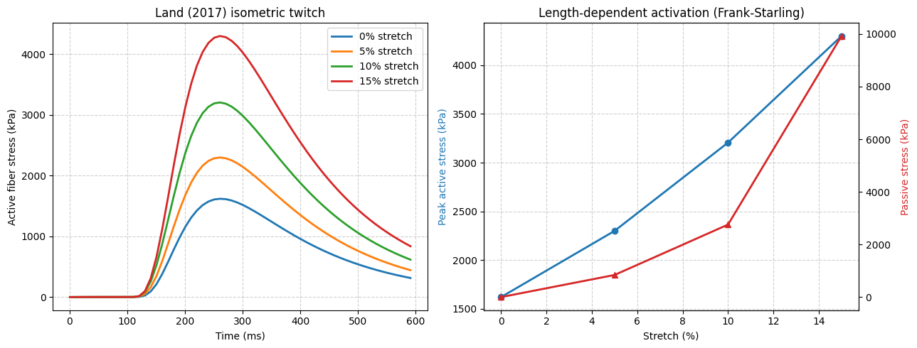
We repeat the twitch at four pre-stretch levels spanning 0-15% strain – the same range as the original demo – and record the full active-stress time course at each.
stretch_amounts = [0.0, 0.5, 1.0, 1.5]  # mm, i.e. 0%, 5%, 10%, 15% strain
strain_pcts = [(s / 10.0) * 100 for s in stretch_amounts]

passive_stresses = []
traces = []

for s, pct in zip(stretch_amounts, strain_pcts):
    p_force, times, active = run_isometric_twitch(s)
    passive_stresses.append(p_force)
    traces.append((times, active))
    print(f"stretch {pct:5.1f}%  passive={p_force:8.4f} kPa  peak active={active.max():8.4f} kPa")
stretch 0.0% passive= 0.0000 kPa peak active=1620.0392 kPa
stretch 5.0% passive=840.7423 kPa peak active=2299.4078 kPa
stretch 10.0% passive=2755.5774 kPa peak active=3206.0444 kPa
stretch 15.0% passive=9921.8714 kPa peak active=4300.3505 kPa
3. Plotting the results#
fig, (ax1, ax2) = plt.subplots(1, 2, figsize=(13, 5))

for (times, active), pct in zip(traces, strain_pcts):
    ax1.plot(times * 1000, active, linewidth=2, label=f"{pct:.0f}% stretch")
ax1.set_xlabel("Time (ms)")
ax1.set_ylabel("Active fiber stress (kPa)")
ax1.set_title("Land (2017) isometric twitch")
ax1.legend()
ax1.grid(True, linestyle="--", alpha=0.6)

peak_active = [active.max() for _, active in traces]
ax2.plot(
    strain_pcts, peak_active, marker="o", linewidth=2, color="tab:blue", label="Peak active stress",
)
ax2b = ax2.twinx()
ax2b.plot(
    strain_pcts, passive_stresses, marker="^", linewidth=2, color="tab:red", label="Passive stress",
)
ax2.set_xlabel("Stretch (%)")
ax2.set_ylabel("Peak active stress (kPa)", color="tab:blue")
ax2b.set_ylabel("Passive stress (kPa)", color="tab:red")
ax2.set_title("Length-dependent activation (Frank-Starling)")
ax2.grid(True, linestyle="--", alpha=0.6)

fig.tight_layout()
plt.show()
4. Conclusion#
Two things fall directly out of the cross-bridge model’s own physics, with no separate length-dependence bolted on:
A real twitch shape. Because activation is driven by an actual calcium transient integrated through troponin binding and cross-bridge kinetics, the active stress rises and relaxes over time – unlike the single-number activation level in the original demo.
Frank-Starling behaviour. Peak active stress increases with pre-stretch purely because
Land2017’sbeta0/beta1gradients make the cross-bridge cycle itself more productive at longer sarcomere lengths – the mechanism lives inside the cell model, not in a hand-fitted multiplier applied afterwards.
See the comparison demo for how this compares
to Lewalle2024, RDQ18 and RDQ20MF.
References#
Sander Land, So-Jin Park-Holohan, Nicolas P Smith, Cristobal G Dos Remedios, Jonathan C Kentish, and Steven A Niederer. A model of cardiac contraction based on novel measurements of tension development in human cardiomyocytes. Journal of molecular and cellular cardiology, 106:68–83, 2017. doi:10.1016/j.yjmcc.2017.03.008.
Francesco Regazzoni and Alfio Quarteroni. An oscillation-free fully staggered algorithm for velocity-dependent active models of cardiac mechanics. Computer Methods in Applied Mechanics and Engineering, 373:113506, 2021. doi:10.1016/j.cma.2020.113506.