Generating UFL for use with FEniCSx#
Most of gotranx’s backends generate code that steps an ODE forward in time: you
get a rhs that works on numpy arrays, and you drive it from a Python loop. The UFL
backend generates UFL expressions instead, which is
the symbolic language FEniCSx uses to write variational
forms.
This is useful when the ODE is coupled to a PDE you are solving with FEniCSx. You
can step the ODE on its own and exchange values with the PDE solver every timestep,
or you can put the ODE unknowns into the same nonlinear system as the PDE unknowns
and solve for all of them at once. The second option needs the Jacobian of the ODE,
including the terms that couple it to the PDE. UFL expressions can be differentiated
with ufl.diff, so you do not have to write that Jacobian yourself.
We use only ufl below, so there is no mesh and no assembly. The example is about
generating the expressions and differentiating them.
Note
UFL is a smaller language than Python’s math. It has no floor, ceiling or
Mod, so an .ode file using any of those cannot be translated to UFL. At the
moment that shows up as a KeyError from inside sympy rather than a proper error
message. If you need something periodic, such as a cardiac activation phase, compute
it outside the model and pass it in. It depends only on time and not on any of the
unknowns, so there is nothing to differentiate anyway.
from pathlib import Path
from typing import Any
import matplotlib.pyplot as plt
import numpy as np
import ufl
from ufl.algorithms.apply_derivatives import apply_derivatives
import gotranx
import gotranx.cli.gotran2py
import gotranx.cli.gotran2ufl
from gotranx.codegen.python import Format
The model#
A two-element Windkessel afterload, fed by a single cardiac chamber through two valves. There are two states, the arterial pressure \(p_{ar}\) and the chamber volume \(V_{lv}\):
The valves are smooth diodes. ContinuousConditional blends between the open and
the shut resistance with a sigmoid, and sigma controls how sharp that blend is. We
use it rather than a hard switch because we are going to differentiate the model,
and a hard switch has no derivative worth having.
The chamber pressure is defined in a component of its own, which is what lets us remove it later on.
ode_str = """
parameters("circulation",
    C_ar = 1.5,      # arterial compliance [mL/mmHg]
    R_sys = 1.0,     # systemic resistance [mmHg s/mL]
    R_open = 0.05,   # valve resistance when open [mmHg s/mL]
    R_shut = 20.0,   # valve resistance when shut [mmHg s/mL]
    sigma = 0.5,     # diode sharpness, smaller is sharper
    p_ven = 12.0     # venous filling pressure [mmHg]
)
states("circulation", p_ar = 60.0, V_lv = 120.0)

parameters("chamber",
    E_min = 0.05,    # minimum (diastolic) elastance [mmHg/mL]
    E_max = 2.5,     # maximum (systolic) elastance [mmHg/mL]
    TC = 0.3,        # contraction duration [s]
    V_0 = 10.0       # unstressed volume [mL]
)

expressions("chamber")
act = Conditional(Lt(t, TC), 0.5 * (1 - cos(pi * t / TC)), 0.0)
E = E_min + (E_max - E_min) * act
p_lv = E * (V_lv - V_0)

expressions("circulation")
R_ao = ContinuousConditional(Gt(p_lv, p_ar), R_open, R_shut, sigma)
R_mi = ContinuousConditional(Gt(p_ven, p_lv), R_open, R_shut, sigma)
Q_ao = (p_lv - p_ar) / R_ao
Q_mi = (p_ven - p_lv) / R_mi

dV_lv_dt = Q_mi - Q_ao
dp_ar_dt = (Q_ao - p_ar / R_sys) / C_ar
"""
ode_file = Path("windkessel.ode")
ode_file.write_text(ode_str)
ode = gotranx.load_ode(ode_file)
2026-10-25 17:16:29 [info ] Load ode windkessel.ode
2026-10-25 17:16:30 [info ] Num states 2
2026-10-25 17:16:30 [info ] Num parameters 10
Note that every symbol is declared. Using a symbol without defining it raises
MissingSymbolError; it is not a way of marking it as an input. Missing variables
come from splitting the model up, which we do next.
print("components:", [c.name for c in ode.components])
print("states:", [s.name for s in ode.states])
components: ['circulation', 'chamber']
states: ['V_lv', 'p_ar']
Splitting the chamber out#
Subtracting a component returns the rest of the ODE. Anything the remainder still uses but no longer defines becomes a missing variable, which the generated code takes as an argument instead of computing.
circuit = ode - ode.get_component("chamber")
print("circuit states :", [s.name for s in circuit.states])
print("circuit missing:", circuit.missing_variables)
circuit states : ['V_lv', 'p_ar']
circuit missing: {'p_lv': 0}
The circuit now expects p_lv from outside. In a coupled simulation this is where a
3D mechanics solver would go, since it is the mechanics, and not an elastance
formula, that decides what pressure the chamber develops at a given volume.
Generating both backends#
We generate UFL and plain numpy from the same ODE object. Having the numpy version
around gives us something to check the UFL version against.
code_ufl = gotranx.cli.gotran2ufl.get_code(circuit, format=Format.none)
code_np = gotranx.cli.gotran2py.get_code(circuit, format=Format.none)
We exec the code into a dictionary rather than writing it to a file, so there is
no generated module lying around to go stale, and nothing to clash if two processes
run at the same time.
model_ufl: dict[str, Any] = {}
model_np: dict[str, Any] = {}
exec(code_ufl, model_ufl)
exec(code_np, model_np)
for line in code_ufl.splitlines():
    if line.startswith("def rhs"):
        print("generated:", line)
generated: def rhs(t, states, parameters, missing_variables):
Warning
gotranx sorts states, parameters and missing variables alphabetically, which is
usually not the order they were declared in. Below, p_ar is index 0 and V_lv is
index 1, the opposite of the states(...) line. Use state_index(name) and
missing_index(name) instead of hard-coding positions, or you will read the wrong
quantity without getting an error.
i_p_ar = model_ufl["state_index"]("p_ar")
i_V_lv = model_ufl["state_index"]("V_lv")
i_p_lv = model_ufl["missing_index"]("p_lv")
print(f"state_index: p_ar={i_p_ar}, V_lv={i_V_lv}   missing_index: p_lv={i_p_lv}")
state_index: p_ar=0, V_lv=1 missing_index: p_lv=0
parameters = model_ufl["init_parameter_values"]()
y0 = model_ufl["init_state_values"]()
Calling the generated rhs#
The generated rhs returns a list of scalar UFL expressions, one per state
derivative, in state_index order. It does not care what its arguments are as long
as they support arithmetic, so we pass ufl.variables: symbolic scalars that
ufl.diff knows how to differentiate with respect to.
In a FEniCSx program these would be Functions, or components of a mixed function,
and each of the returned expressions would become one row of a block residual.
t_val = 0.15
p_lv_val = 55.0
states_sym = [ufl.variable(ufl.as_ufl(float(v))) for v in y0]
p_lv_sym = ufl.variable(ufl.as_ufl(p_lv_val))
rows = model_ufl["rhs"](t_val, states_sym, parameters, [p_lv_sym])
print(f"rhs returned {len(rows)} scalar UFL expressions")
print("dp_ar/dt =", rows[i_p_ar])
rhs returned 2 scalar UFL expressions
dp_ar/dt = (-1 * (var0(60.0)) + ((var2(55.0)) + -1 * (var0(60.0))) / (0.05 * (1 + -1 * 1 / (1 + exp(((var2(55.0)) + -1 * (var0(60.0))) / 0.5))) + 20.0 / (1 + exp(((var2(55.0)) + -1 * (var0(60.0))) / 0.5)))) / 1.5
A UFL expression can be evaluated if you supply a value for every variable in it, so we can compare the two backends directly.
subs = {v: float(val) for v, val in zip(states_sym, y0)}
subs[p_lv_sym] = p_lv_val
f_ufl = np.array([float(r((), subs)) for r in rows])
f_np = np.asarray(model_np["rhs"](t_val, y0, parameters, np.array([p_lv_val])))
print("f (ufl)  =", f_ufl)
print("f (numpy)=", f_np)
print("max abs difference:", np.max(np.abs(f_ufl - f_np)))
f (ufl)  = [-40.16667421  -1.89998868]
f (numpy)= [-40.16667421  -1.89998868]
max abs difference: 0.0
Differentiating the generated expressions#
ufl.diff differentiates them symbolically, so the Jacobian is exact and there is
no separate formula to keep in step with the model.
J = np.array(
    [[float(apply_derivatives(ufl.diff(r, s))((), subs)) for s in states_sym] for r in rows],
)
print("dF/dy =\n", J)
dF/dy =
 [[-0.69998641  0.        ]
 [ 0.04997962  0.        ]]
Compare against central differences on the numpy backend.
h = 1e-6
J_fd = np.zeros_like(J)
for j in range(len(y0)):
    yp, ym = np.array(y0, dtype=float), np.array(y0, dtype=float)
    yp[j] += h
    ym[j] -= h
    J_fd[:, j] = (
        np.asarray(model_np["rhs"](t_val, yp, parameters, np.array([p_lv_val])))
        - np.asarray(model_np["rhs"](t_val, ym, parameters, np.array([p_lv_val])))
    ) / (2 * h)
print("max |J_symbolic - J_finite_difference| =", np.max(np.abs(J - J_fd)))
max |J_symbolic - J_finite_difference| = 1.423459128346849e-09
The \(\partial/\partial V_{lv}\) column is zero. After the split, \(V_{lv}\) does not appear in the circuit equations at all. It acts only through \(p_{lv}\), which now comes from outside.
So the derivative with respect to the missing variable is the interesting one. It is the coupling sensitivity, and it is what you need if you want to solve the ODE together with whatever supplies \(p_{lv}\).
dF_dp_lv = np.array(
    [float(apply_derivatives(ufl.diff(r, p_lv_sym))((), subs)) for r in rows],
)
print("dF/dp_lv =", dF_dp_lv)
dF/dp_lv = [ 0.03331975 -0.09997962]
Stepping the model#
To put the pieces together, we solve the circuit with backward Euler and take the Newton Jacobian from the symbolic derivatives above. Implicit stepping is the usual reason to want a Jacobian in the first place: with sharp valves, an explicit scheme needs a very small step to stay stable.
p_lv has to come from somewhere, so we use the elastance closure we removed,
evaluated in Python. That also gives us a periodic phase without needing Mod
inside the model.
Its parameters are no longer in the circuit’s parameter array, since they were removed along with the closure, so the stand-in carries its own values the way an external solver would.
def chamber_pressure(t: float, V_lv: float, beat: float = 1.0) -> float:
    """The closure we split out, standing in for an external solver."""
    E_min, E_max, TC, V_0 = 0.05, 2.5, 0.3, 10.0
    phase = t % beat  # periodic in Python, where `Mod` is available
    act = 0.5 * (1 - np.cos(np.pi * phase / TC)) if phase < TC else 0.0
    return (E_min + (E_max - E_min) * act) * (V_lv - V_0)
def backward_euler_step(t_new: float, y_old: np.ndarray, dt: float) -> np.ndarray:
    """One backward-Euler step, Newton-solved with the symbolic Jacobian."""
    y = y_old.copy()
    for _ in range(50):
        p_lv = chamber_pressure(t_new, float(y[i_V_lv]))

        sym = [ufl.variable(ufl.as_ufl(float(v))) for v in y]
        p_sym = ufl.variable(ufl.as_ufl(p_lv))
        r = model_ufl["rhs"](t_new, sym, parameters, [p_sym])
        at = {v: float(val) for v, val in zip(sym, y)}
        at[p_sym] = p_lv

        f = np.array([float(ri((), at)) for ri in r])
        df_dy = np.array(
            [[float(apply_derivatives(ufl.diff(ri, s))((), at)) for s in sym] for ri in r],
        )

        residual = y - y_old - dt * f
        if np.max(np.abs(residual)) < 1e-10:
            break
        y -= np.linalg.solve(np.eye(len(y)) - dt * df_dy, residual)
    return y
The initial state is not on the limit cycle, and this circuit is open: it drains to a sink and refills from a fixed pressure. We run six beats and let it settle.
dt = 0.002
times = np.arange(0.0, 6.0, dt)
history = np.zeros((times.size, len(y0)))
y = np.array(y0, dtype=float)
for k, t_k in enumerate(times):
    y = backward_euler_step(t_k + dt, y, dt)
    history[k] = y
p_lv_trace = np.array(
    [chamber_pressure(t_k, V) for t_k, V in zip(times, history[:, i_V_lv])],
)
fig, (ax1, ax2) = plt.subplots(1, 2, figsize=(11, 4.2), layout="constrained")
ax1.plot(times, p_lv_trace, label="$p_{lv}$")
ax1.plot(times, history[:, i_p_ar], label="$p_{ar}$")
ax1.set_xlabel("Time [s]")
ax1.set_ylabel("Pressure [mmHg]")
ax1.legend()
ax1.set_title("Pressures")
ax2.plot(history[:, i_V_lv], p_lv_trace, linewidth=0.9)
ax2.set_xlabel("$V_{lv}$ [mL]")
ax2.set_ylabel("$p_{lv}$ [mmHg]")
ax2.set_title("Pressure-volume loop")
Text(0.5, 1.0, 'Pressure-volume loop')
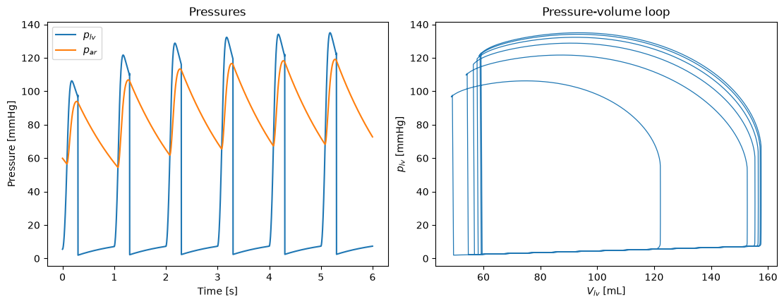
fig.savefig("ufl_backend.png", dpi=140)
Summary#
gotranx.cli.gotran2uflgives you arhsreturning a list of scalar UFL expressions, one per state derivative, instate_indexorder.Splitting out a component turns everything the remainder no longer defines into a missing variable, which makes a convenient seam for coupling to another solver.
ufl.diffdifferentiates with respect to states and missing variables alike. The derivatives with respect to missing variables are the coupling terms.Generating the numpy backend from the same model gives you a cheap reference to check the UFL against.
Index by name rather than by position, since the generated ordering is alphabetical.
UFL has no
floor,ceilingorMod.