Premature Ventricular Complexes (PVCs)#
In this demo we try to replicate the experimental setup conducted in [ZLH+21]
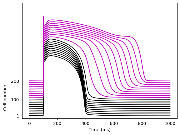
We simulate a 1D “cable” of tissue with a detailed ionic current model (ten Tusscher–Panfilov 2006), a scalar conductivity/diffusion coefficient \(M\), and a region of reduced repolarization reserve (the rapid delayed rectifier and slow delayed rectifier conductances \(g_{Kr}\) and \(g_{Ks}\) are set to zero in the right half of the cable). When all cells are stimulated simultaneously with a periodic stimulus \(I_{stim}\), the heterogeneity in repolarization can, under the right conditions, give rise to a premature ventricular complex (PVC) — an ectopic beat originating from the heterogeneous region rather than from the (here, simultaneous) normal activation. See the mathematical background page for the monodomain model and notation used below, and the pacing train demo for the same tissue setup with a different (single-point, rapid) pacing protocol.
First we do the necessary imports
Next we set the output directory for the results and define the geometry. Here we specify an interval mesh of 200 cells with 0.015 cm between each cell
here = Path.cwd()
outdir = here / "results-pvc"
mesh_unit = "cm"
dx = 0.015
num_cells = 200
L = num_cells * dx
comm = MPI.COMM_WORLD
mesh = dolfinx.mesh.create_interval(comm, num_cells, (0, L))
We will use the tensusscher panfilov model
model_path = Path("tentusscher_panfilov_2006_epi_cell.py")
if not model_path.is_file():
    here = Path.cwd()
    cell_ode = gotranx.load_ode(
        here
        / ".."
        / "odes"
        / "tentusscher_panfilov_2006"
        / "tentusscher_panfilov_2006_epi_cell.ode",
    )
    code = gotranx.cli.gotran2py.get_code(
        cell_ode,
        scheme=[gotranx.schemes.Scheme.generalized_rush_larsen],
    )
    model_path.write_text(code)
import tentusscher_panfilov_2006_epi_cell
model = tentusscher_panfilov_2006_epi_cell.__dict__
# Change this to run the simulations for longer
end_time = 1000.0
We specify a diffusion coefficient \(D\) and a membrane capacitance \(C_m\). Since the cable is 1D we use \(D\) directly as the (scalar) conductivity \(M\) below.
D = beat.units.ureg.Quantity(0.0005, "cm**2 / ms")
Cm = beat.units.ureg.Quantity(1.0, "uF/cm**2")
Next we run a single cell model with the to get the correct steady state solutions. We run this for 50 beats with a stimulation every 1000.0 ms
parameters = model["init_parameter_values"](stim_period=1000.0)
dt = 0.01
nbeats = 50
fun = model["generalized_rush_larsen"]
y = get_steady_state(
    fun=fun,
    init_states=model["init_state_values"](),
    parameters=parameters,
    outdir=outdir / "prebeats",
    BCL=500,
    nbeats=nbeats,
    track_indices=[model["state_index"]("V"), model["state_index"]("Ca_i")],
    dt=dt,
)
# -
Now we create the stimulus current which is 0.0 is we stimulate all the cells at once (in which case the stimulation is applied directly to all cells).
time = dolfinx.fem.Constant(mesh, 0.0)
I_s = dolfinx.fem.Constant(mesh, 0.0)
We start the stimulation after 100 ms with period of 1000 ms
parameters = model["init_parameter_values"](stim_start=100.0, stim_period=1000)
Now we would like to change the conductances for the cells in the right most part of the cable. We choose a first order Lagrange space for this, so that we have one set of parameters for each cells, and then we copy over the default parameters
V_ode = dolfinx.fem.functionspace(mesh, ("Lagrange", 1))
parameters_ode = np.zeros(
    (len(parameters), V_ode.dofmap.index_map.size_local),
    dtype=np.float64,
)
parameters_ode.T[:] = parameters
To set the values of the parameters we first need to get the coordinates of the cells which we can do using the ufl.SpatialCoordinate function
Next we set the values og \(g_Kr\) function
g_Kr_index = model["parameter_index"]("g_Kr")
g_Kr_value = parameters[g_Kr_index]
g_Kr = dolfinx.fem.Function(V_ode)
We interpolate the values to the function space using a conditional expression
g_Kr.interpolate(
    dolfinx.fem.Expression(
        ufl.conditional(ufl.ge(X[0], L / 2), 0.0, g_Kr_value),
        beat.utils.interpolation_points(V_ode),
    ),
)
and set the values in the parameters array
parameters_ode[g_Kr_index, :] = g_Kr.x.array
and similar for the conductance \(g_Ks\)
g_Ks_index = model["parameter_index"]("g_Ks")
g_Ks_value = parameters[g_Ks_index]
g_Ks = dolfinx.fem.Function(V_ode)
g_Ks.interpolate(
    dolfinx.fem.Expression(
        ufl.conditional(ufl.ge(X[0], L / 2), 0.0, g_Ks_value),
        beat.utils.interpolation_points(V_ode),
    ),
)
parameters_ode[g_Ks_index, :] = g_Ks.x.array
Finally we set up the PDE and ODE models and combine them with the (default \(\theta = 1\), Godunov-split) splitting solver.
pde = beat.MonodomainModel(
    time=time,
    mesh=mesh,
    M=D.magnitude,
    I_s=I_s,
    C_m=Cm.magnitude,
)
ode = beat.odesolver.DolfinODESolver(
    v_ode=dolfinx.fem.Function(V_ode),
    v_pde=pde.state,
    fun=fun,
    init_states=y,
    parameters=parameters_ode,
    num_states=len(y),
    v_index=model["state_index"]("V"),
)
solver = beat.MonodomainSplittingSolver(pde=pde, ode=ode)

checkpointfname = outdir / "pvc_checkpoint.bp"

shutil.rmtree(checkpointfname, ignore_errors=True)
io4dolfinx.write_mesh(checkpointfname, mesh)


def save(t):
    v = solver.pde.v.x.array
    if t % 100.0 == 0:
        print(f"Solve for {t=:.2f}, {v.max() =}, {v.min() =}")
    io4dolfinx.write_function(checkpointfname, solver.pde.v, time=t, name="v")
and solve it
t = 0.0
save_freq = int(1.0 / dt)
i = 0
done_stimulating = False
while t < end_time + 1e-12:

    if i % save_freq == 0:
        save(t)
    solver.step((t, t + dt))
    i += 1
    t += dt
Solve for t=0.00, v.max() =np.float64(-84.95148875708807), v.min() =np.float64(-84.95148875708807)
def post_process(dx, outdir):
    mesh = io4dolfinx.read_mesh(comm=comm, filename=checkpointfname)
    V = dolfinx.fem.functionspace(mesh, ("P", 1))
    v = dolfinx.fem.Function(V)
    times = io4dolfinx.read_timestamps(comm=comm, filename=checkpointfname, function_name="v")

    cellnr = [0, 25, 50, 75, 100, 125, 150, 175, 200]
    cellnr = np.arange(0, 200, 10)

    p1 = 25 * dx
    p2 = 175 * dx
    dp = 150 * dx * beat.units.ureg("cm")
    tp1 = np.inf
    tp2 = np.inf

    points = cellnr * dx
    p1p2 = [p1, p2]

    if not (outdir / "traces.npy").is_file():
        traces = np.zeros((len(times), len(cellnr)))

        for i, ti in enumerate(times):
            io4dolfinx.read_function(checkpointfname, v, time=ti, name="v")

            traces[i, :] = scifem.evaluate_function(
                v,
                np.expand_dims(points, 1),
            ).squeeze()
            vp1p2 = scifem.evaluate_function(v, np.expand_dims(p1p2, 1)).squeeze()

            if vp1p2[0] > 0.0 and tp1 == np.inf:
                tp1 = ti
            if vp1p2[0] > 0.0 and tp2 == np.inf:
                tp2 = ti

        np.save(outdir / "traces.npy", traces)
        np.save(outdir / "times.npy", times)
        (outdir / "cv.text").write_text(f"{tp1} {tp2}")

    traces = np.load(outdir / "traces.npy")
    t = np.load(outdir / "times.npy")
    tp1, tp2 = np.loadtxt(outdir / "cv.text")
    tp1 *= beat.units.ureg("ms")
    tp2 *= beat.units.ureg("ms")

    if not np.isclose(tp1, tp2):
        cv = dp / (tp2 - tp1)
        print(
            f"Conduction velocity:: {cv.to('cm/ms').magnitude} cm/ms "
            f"= {cv.to('m/s').magnitude} m/s",
        )

    # Plot 3D plot for all traces
    fig, ax = plt.subplots()
    for i, cell_index in enumerate(cellnr):
        color = "k" if cell_index < 100 else "m"
        ax.plot(t, cell_index / 3 * np.ones_like(t) + traces[:, i], color=color)
    ax.set_xlabel("Time (ms)")
    ax.set_yticks([-22, -55, -85])
    ax.set_yticklabels([200, 100, 1])
    fig.text(x=0.03, y=0.17, s="Cell number", rotation=90)

    ax.set_ylim(-90, 120)
    fig.savefig(outdir / "V_3d.png")
post_process(dx, outdir)