Conduction velocity and ECG for slabs

In this demo we will show how to compute conduction velocity and ECG for a Slab geometry.

This demo introduces the full “realistic” workflow used by most of the other tissue-level demos in this repository: a detailed ionic current model (here ToR-ORd) with different parameters for the endocardial, mid-myocardial and epicardial layers of the tissue, a physically motivated conductivity tensor \(M\) built from fibre directions and literature conductivity values, and a stimulus current \(I_{stim}\) applied at one end of a thin slab of tissue to trigger a propagating wave. Once we have simulated the transmembrane potential \(v\) over time, we measure how fast the depolarization wave travels (the conduction velocity) and recover a pseudo-ECG signal from the simulated \(v\) using beat.ecg.ECGRecovery. See the mathematical background page for the monodomain model and notation used below, and the left-ventricle demo for a more detailed walk-through of the same building blocks (steady-state initial conditions, multi-layer cell models, conductivity tensors, and the splitting solver).

from pathlib import Path
import shutil
from mpi4py import MPI

import io4dolfinx

import dolfinx
import matplotlib.pyplot as plt
import numpy as np
import gotranx
import scifem
import beat
import pyvista
from dolfinx.io import VTXMeshPolicy

from beat.geometry import Geometry

comm = MPI.COMM_WORLD
results_folder = Path("results-slab")
results_folder.mkdir(exist_ok=True)
save_every_ms = 1.0

transverse = False
end_time = 20.0
dt = 0.05
overwrite = False
stim_amp = 5000.0
mesh_unit = "cm"
dx = 0.05 * beat.units.ureg("cm").to(mesh_unit).magnitude
L = 1.0 * beat.units.ureg("cm").to(mesh_unit).magnitude
mesh = beat.geometry.get_3D_slab_mesh(comm=comm, Lx=L, Ly=dx, Lz=dx, dx=dx / 5)

tol = 1.0e-8

marker = 1

def S1_subdomain(x):
    return x[0] <= tol

facets = dolfinx.mesh.locate_entities_boundary(
    mesh,
    mesh.topology.dim - 1,
    S1_subdomain,
)
ffun = dolfinx.mesh.meshtags(
    mesh,
    mesh.topology.dim - 1,
    facets,
    np.full(len(facets), marker, dtype=np.int32),
)

V = dolfinx.fem.functionspace(mesh, ("P", 1))

plotter_markers = pyvista.Plotter()
grid = pyvista.UnstructuredGrid(*dolfinx.plot.vtk_mesh(V))
plotter_markers.add_mesh(grid, show_edges=True)
if mesh.geometry.dim == 2:
    plotter_markers.view_xy()

2026-08-11 14:28:35.864 (   0.542s) [    7FCE52BDC140]vtkXOpenGLRenderWindow.:1460  WARN| bad X server connection. DISPLAY=

if not pyvista.OFF_SCREEN:
    plotter_markers.show()
else:
    plotter_markers.screenshot(results_folder / "markers.png")

def endo_epi(x):
    return np.where(x[0] < L / 3, 1, np.where(x[0] > 2 * L / 3, 2, 0))

cfun_func = dolfinx.fem.Function(V)
cfun_func.interpolate(endo_epi)

plotter_markers = pyvista.Plotter()
grid = pyvista.UnstructuredGrid(*dolfinx.plot.vtk_mesh(V))
grid.point_data["V"] = cfun_func.x.array
plotter_markers.add_mesh(grid, show_edges=True)
if mesh.geometry.dim == 2:
    plotter_markers.view_xy()

if not pyvista.OFF_SCREEN:
    plotter_markers.show()
else:
    plotter_markers.screenshot(results_folder / "endo_epi.png")

with dolfinx.io.XDMFFile(comm, results_folder / "ffun.xdmf", "w") as xdmf:
    xdmf.write_mesh(mesh)
    xdmf.write_meshtags(ffun, mesh.geometry)

with dolfinx.io.XDMFFile(comm, results_folder / "endo_epi.xdmf", "w") as xdmf:
    xdmf.write_mesh(mesh)
    xdmf.write_function(cfun_func)

g_il = 0.16069
g_el = 0.625
g_it = 0.04258
g_et = 0.236

f0, s0, n0 = beat.geometry.get_3D_slab_microstructure(mesh, transverse)

markers = {"ENDO": (marker, 2)}

data = Geometry(
    mesh=mesh,
    ffun=ffun,
    markers=markers,
    f0=f0,
    s0=s0,
    n0=n0,
)
save_freq = round(save_every_ms / dt)

print("Running model")
# Load the model
model_path = Path("ToRORd_dynCl_endo.py")
if not model_path.is_file():
    print("Generate code for cell model")
    here = Path.cwd()
    ode = gotranx.load_ode(here / ".." / "odes" / "torord" / "ToRORd_dynCl_endo.ode")
    code = gotranx.cli.gotran2py.get_code(
        ode,
        scheme=[gotranx.schemes.Scheme.generalized_rush_larsen],
    )
    model_path.write_text(code)

Running model

import ToRORd_dynCl_endo

model = ToRORd_dynCl_endo.__dict__

Surface to volume ratio \(\chi\)

chi = 1400.0 * beat.units.ureg("cm**-1")

Membrane capacitance \(C_m\)

C_m = 1.0 * beat.units.ureg("uF/cm**2")

print("Get steady states")
nbeats = 2  # Should be set to at least 200
init_states = {
    0: beat.single_cell.get_steady_state(
        fun=model["generalized_rush_larsen"],
        init_states=model["init_state_values"](),
        parameters=model["init_parameter_values"](celltype=2),
        outdir=results_folder / "mid",
        BCL=1000,
        nbeats=nbeats,
        track_indices=[model["state_index"]("v"), model["state_index"]("cai")],
        dt=0.05,
    ),
    1: beat.single_cell.get_steady_state(
        fun=model["generalized_rush_larsen"],
        init_states=model["init_state_values"](),
        parameters=model["init_parameter_values"](celltype=0),
        outdir=results_folder / "endo",
        BCL=1000,
        nbeats=nbeats,
        track_indices=[
            model["state_index"]("v"),
            model["state_index"]("cai"),
            model["state_index"]("nai"),
        ],
        dt=0.05,
    ),
    2: beat.single_cell.get_steady_state(
        fun=model["generalized_rush_larsen"],
        init_states=model["init_state_values"](),
        parameters=model["init_parameter_values"](celltype=1),
        outdir=results_folder / "epi",
        BCL=1000,
        nbeats=nbeats,
        track_indices=[model["state_index"]("v"), model["state_index"]("cai")],
        dt=0.05,
    ),
}
# endo = 0, epi = 1, M = 2
parameters = {
    0: model["init_parameter_values"](i_Stim_Amplitude=0.0, celltype=2),
    1: model["init_parameter_values"](i_Stim_Amplitude=0.0, celltype=0),
    2: model["init_parameter_values"](i_Stim_Amplitude=0.0, celltype=1),
}
fun = {
    0: model["generalized_rush_larsen"],
    1: model["generalized_rush_larsen"],
    2: model["generalized_rush_larsen"],
}
v_index = {
    0: model["state_index"]("v"),
    1: model["state_index"]("v"),
    2: model["state_index"]("v"),
}

Get steady states

The stimulus current \(I_{stim}\) is applied at the endocardial (ENDO) face of the slab, and is already divided by \(\chi\) internally by define_stimulus so that it can be added directly to the right-hand side of the monodomain equation, see the mathematical background page.

time = dolfinx.fem.Constant(mesh, dolfinx.default_scalar_type(0.0))
assert data.ffun is not None
I_s = beat.stimulation.define_stimulus(
    mesh=data.mesh,
    chi=chi,
    time=time,
    subdomain_data=data.ffun,
    marker=markers["ENDO"][0],
    amplitude=stim_amp,
    mesh_unit=mesh_unit,
)

fiber_direction = data.f0
assert fiber_direction is not None

The effective (monodomain) conductivity tensor \(M\) is built from the intracellular/extracellular conductivities g_il, g_it, g_el, g_et along and across the fibre direction, harmonic-averaged and divided by \(\chi\) so that it matches the equation in the mathematical background page.

M = beat.conductivities.define_conductivity_tensor(
    chi,
    f0=fiber_direction,
    g_il=g_il,
    g_it=g_it,
    g_el=g_el,
    g_et=g_et,
)

params = {"preconditioner": "sor", "use_custom_preconditioner": False}
pde = beat.MonodomainModel(
    time=time,
    mesh=data.mesh,
    M=M,
    I_s=I_s,
    params=params,
    C_m=C_m.to(f"uF/{mesh_unit}**2").magnitude,
)

V_ode = dolfinx.fem.functionspace(data.mesh, ("P", 1))
ode = beat.odesolver.DolfinMultiODESolver(
    v_ode=dolfinx.fem.Function(V_ode),
    v_pde=pde.state,
    markers=cfun_func,
    num_states={i: len(s) for i, s in init_states.items()},
    fun=fun,
    init_states=init_states,
    parameters=parameters,
    v_index=v_index,
)
# Combine the PDE and (multi-region) ODE solver with a splitting solver. We use the default
# $\theta = 1$, i.e. (first-order) Godunov splitting.

t = 0.0
solver = beat.MonodomainSplittingSolver(pde=pde, ode=ode)

vtxfname = results_folder / "slab.bp"
checkpointfname = results_folder / "slab_checkpoint.bp"

shutil.rmtree(vtxfname, ignore_errors=True)
shutil.rmtree(checkpointfname, ignore_errors=True)
vtx = dolfinx.io.VTXWriter(
    comm,
    vtxfname,
    [solver.pde.state],
    engine="BP4",
    mesh_policy=VTXMeshPolicy.reuse,
)

io4dolfinx.write_mesh(checkpointfname, mesh)

def save(t):
    v = solver.pde.state.x.array
    print(f"Solve for {t=:.2f}, {v.max() =}, {v.min() =}")
    vtx.write(t)
    io4dolfinx.write_function(checkpointfname, solver.pde.state, time=t, name="v")

i = 0
while t < end_time + 1e-12:
    # Make sure to save at the same time steps that is used by Ambit

    if i % save_freq == 0:
        save(t)

    solver.step((t, t + dt))
    i += 1
    t += dt

Solve for t=0.00, v.max() =np.float64(-89.49461598667106), v.min() =np.float64(-89.84978422825839)

Solve for t=1.00, v.max() =np.float64(96.18090213247223), v.min() =np.float64(-89.84982993061158)

Solve for t=2.00, v.max() =np.float64(156.7317581652501), v.min() =np.float64(-89.8498672815758)

Solve for t=3.00, v.max() =np.float64(60.93322179874107), v.min() =np.float64(-89.84990772868004)

Solve for t=4.00, v.max() =np.float64(40.046999771428986), v.min() =np.float64(-89.8499384314671)

Solve for t=5.00, v.max() =np.float64(30.118531218608), v.min() =np.float64(-89.8499353942576)

Solve for t=6.00, v.max() =np.float64(25.25918861495623), v.min() =np.float64(-89.84988046329886)

Solve for t=7.00, v.max() =np.float64(22.822875687583092), v.min() =np.float64(-89.8497745953058)

Solve for t=8.00, v.max() =np.float64(22.08346742786114), v.min() =np.float64(-89.84963217201073)

Solve for t=9.00, v.max() =np.float64(22.86740070084043), v.min() =np.float64(-89.84947134388037)

Solve for t=10.00, v.max() =np.float64(23.239979893675116), v.min() =np.float64(-89.84930799847754)

Solve for t=11.00, v.max() =np.float64(23.3322047847248), v.min() =np.float64(-89.84915356790438)

Solve for t=12.00, v.max() =np.float64(23.35188241485754), v.min() =np.float64(-89.84901503532018)

Solve for t=13.00, v.max() =np.float64(23.356830164032143), v.min() =np.float64(-89.84889571425754)

Solve for t=14.00, v.max() =np.float64(23.35401951196897), v.min() =np.float64(-89.84879224671721)

Solve for t=15.00, v.max() =np.float64(22.60186854921293), v.min() =np.float64(-89.84854189377153)

Solve for t=16.00, v.max() =np.float64(21.209130923616026), v.min() =np.float64(-89.84179231272114)

Solve for t=17.00, v.max() =np.float64(21.205289594434372), v.min() =np.float64(-89.56313334895438)

Solve for t=18.00, v.max() =np.float64(21.93513100869462), v.min() =np.float64(-76.95721666302443)

Solve for t=19.00, v.max() =np.float64(33.41454207029696), v.min() =np.float64(14.971675112922254)

Solve for t=20.00, v.max() =np.float64(23.465127541523454), v.min() =np.float64(14.17342600820865)

Compute conduction velocity and ECG

threshold = 0.0
x0 = L * 0.25
x1 = L * 0.75
if mesh.geometry.dim == 2:
    p_ecg = (L * 2.0, dx * 0.5)
    p1 = (x0, dx * 0.5)
    p2 = (x1, dx * 0.5)
else:
    p_ecg = (L * 2.0, dx * 0.5, dx * 0.5)  # type: ignore
    p1 = (x0, dx * 0.5, dx * 0.5)  # type: ignore
    p2 = (x1, dx * 0.5, dx * 0.5)  # type: ignore

Need to either save the functions on the input mesh using io4dolfinx.write_function_on_input_mesh or read the mesh again see https://scientificcomputing.github.io/io4dolfinx/docs/original_checkpoint.html

mesh = io4dolfinx.read_mesh(comm=comm, filename=checkpointfname)
V = dolfinx.fem.functionspace(mesh, ("P", 1))
v = dolfinx.fem.Function(V)

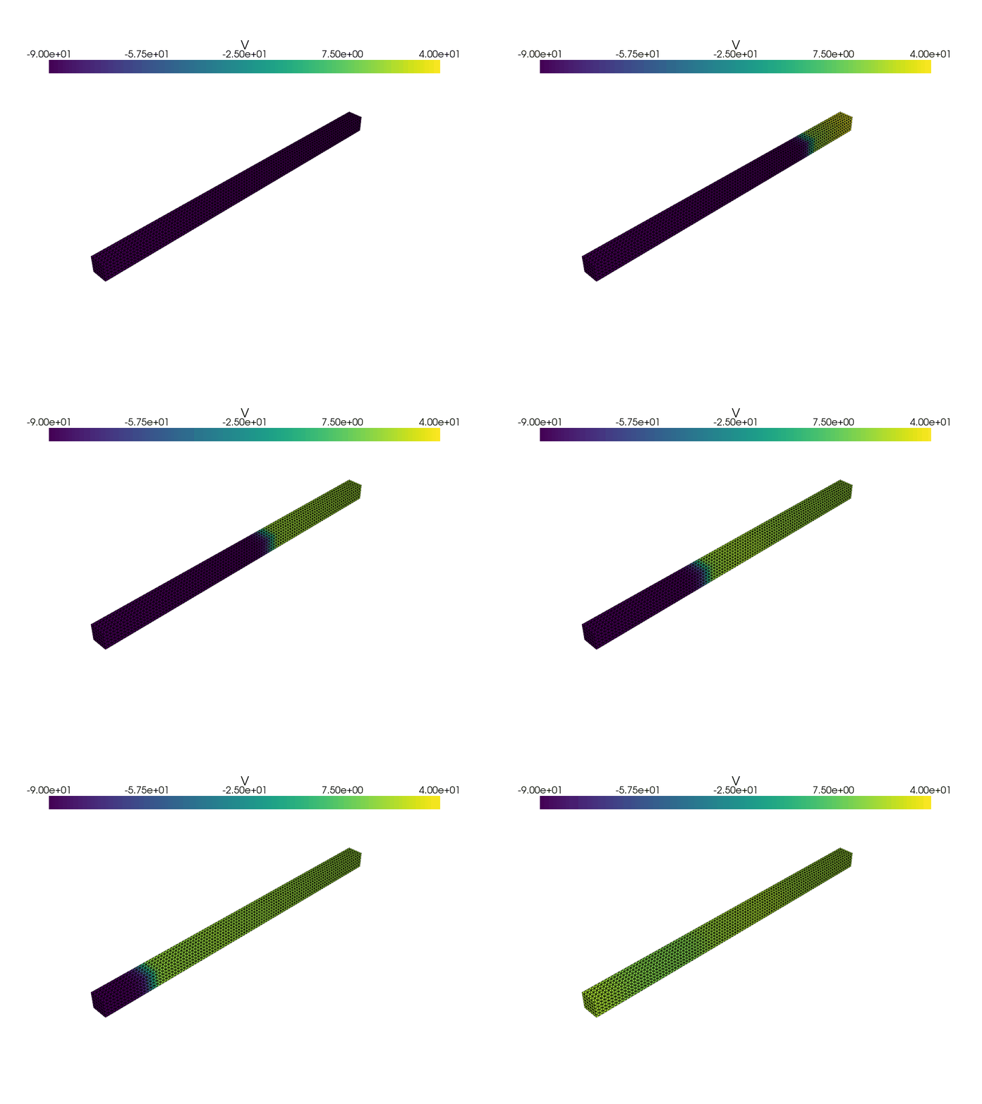
plotter_voltage = pyvista.Plotter()
grid = pyvista.UnstructuredGrid(*dolfinx.plot.vtk_mesh(V))
grid.point_data["V"] = v.x.array
viridis = plt.get_cmap("viridis")
sargs = dict(
    title_font_size=25,
    label_font_size=20,
    fmt="%.2e",
    color="black",
    position_x=0.1,
    position_y=0.8,
    width=0.8,
    height=0.1,
)

plotter_voltage.add_mesh(
    grid,
    show_edges=True,
    lighting=False,
    cmap=viridis,
    scalar_bar_args=sargs,
    clim=[-90.0, 40.0],
)

times = io4dolfinx.read_timestamps(
    comm=comm, filename=checkpointfname, function_name="v",
)
t1 = np.inf
t2 = np.inf
phie = []
ecg = beat.ecg.ECGRecovery(
    v=v,
    sigma_b=1.0,
    C_m=C_m.to(f"uF/{mesh_unit}**2").magnitude,
    M=M,
)
p_ecg_form = ecg.eval(p_ecg)
gif_file = Path("voltage_slab_time.gif")
gif_file.unlink(missing_ok=True)
plotter_voltage.open_gif(gif_file.as_posix())
for t in times:
    io4dolfinx.read_function(checkpointfname, v, time=t, name="v")
    ecg.solve()
    phie.append(
        mesh.comm.allreduce(dolfinx.fem.assemble_scalar(p_ecg_form), op=MPI.SUM),
    )

    grid.point_data["V"] = v.x.array
    plotter_voltage.write_frame()
    v1, v2 = scifem.evaluate_function(v, [p1, p2])
    print(f"Read {t=:.2f}, {v1 =}, {v2 =}")

    if v1 > threshold:
        t1 = min(t, t1)
    if v2 > threshold:
        t2 = min(t, t2)

plotter_voltage.close()

Read t=0.00, v1 =array([-89.74885233]), v2 =array([-89.84978423])
Read t=1.00, v1 =array([-89.74382839]), v2 =array([-89.84285777])
Read t=2.00, v1 =array([-89.73163886]), v2 =array([-89.82798931])
Read t=3.00, v1 =array([-89.61587526]), v2 =array([-89.81826262])

Read t=4.00, v1 =array([-85.62186006]), v2 =array([-89.81229107])
Read t=5.00, v1 =array([-4.60050736]), v2 =array([-89.80853166])
Read t=6.00, v1 =array([21.08622303]), v2 =array([-89.80609628])
Read t=7.00, v1 =array([21.50192394]), v2 =array([-89.80448303])

Read t=8.00, v1 =array([21.44475013]), v2 =array([-89.80339789])
Read t=9.00, v1 =array([21.16412938]), v2 =array([-89.80266036])
Read t=10.00, v1 =array([20.81092625]), v2 =array([-89.80211725])
Read t=11.00, v1 =array([20.43555961]), v2 =array([-89.80027631])

Read t=12.00, v1 =array([20.07549438]), v2 =array([-89.74701865])
Read t=13.00, v1 =array([19.7828611]), v2 =array([-87.92275988])
Read t=14.00, v1 =array([19.60614111]), v2 =array([-32.74283281])
Read t=15.00, v1 =array([19.56103128]), v2 =array([20.28303277])

Read t=16.00, v1 =array([19.63238866]), v2 =array([19.28794502])
Read t=17.00, v1 =array([19.79060021]), v2 =array([17.80693058])
Read t=18.00, v1 =array([20.00495566]), v2 =array([16.3537289])
Read t=19.00, v1 =array([20.25124732]), v2 =array([15.11195494])

Read t=20.00, v1 =array([20.5088712]), v2 =array([14.18767015])

if not np.isclose(t1, t2):
    cv = (x1 - x0) / (t2 - t1) * beat.units.ureg(f"{mesh_unit}/ms")
    msg = (
        f"Conduction velocity = {cv.magnitude:.3f} mm/ms or "  #
        f" {cv.to('m/s').magnitude:.3f} m/s or "  #
        f" {cv.to('cm/s').magnitude:.3f} cm/s"  #
    )
    print(msg)

Conduction velocity = 0.056 mm/ms or  0.556 m/s or  55.556 cm/s

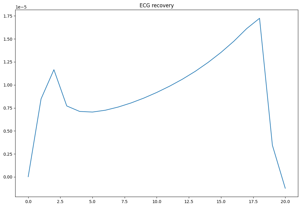
fig, ax = plt.subplots(1, 1, figsize=(12, 8))
ax.plot(times, phie)
ax.set_title("ECG recovery")
fig.savefig(results_folder / "ecg_recovery.png")