Solving a simple ODE

In this example we will show how to solve a simple ODE using the ODE solver in beat. While this is not the main purpose of the package it might be useful to solve the single cell models.

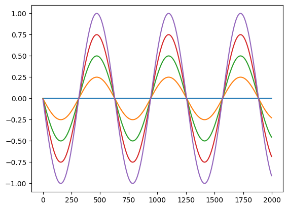
In the context of the mathematical background page, this demo solves only the ODE part of the coupled cell-model system,

\[ \frac{dv}{dt} = -I_{ion}(v, s), \qquad \frac{ds}{dt} = f(v, s), \]

for a toy right-hand side (a simple undamped oscillator with \(I_{ion}(v, s) = s\) and \(f(v, s) = -v\)), at num_points independent points at once, using beat.odesolver.solve with a forward Euler scheme. This is exactly the kind of ODE step that beat.MonodomainSplittingSolver performs at every mesh point during steps 1 and 3 of the operator splitting scheme — here without any PDE step or diffusion coupling in between.

First we import the necessary packages

import numpy as np
from time import perf_counter
import matplotlib.pyplot as plt

import beat

def simple_ode_forward_euler(states, t, dt, parameters):
    v, s = states
    states[0] = v - s * dt
    states[1] = s + v * dt

num_points = 5
num_states = 2
states = np.zeros((num_states, num_points))
states[1, :] = np.linspace(0, 1, num_points)
dt = 0.01
t_bound = 20.0
t0 = 0.0

V_index = 0

nT = int((t_bound - t0) / dt) - 1
V = np.zeros((nT, num_points))
t0 = perf_counter()
beat.odesolver.solve(
    fun=simple_ode_forward_euler,
    t_bound=t_bound,
    states=states,
    V=V,
    V_index=V_index,
    dt=dt,
    parameters=None,
)

fig, ax = plt.subplots()
for i in range(num_points):
    ax.plot(V[:, i])
fig.savefig("simple.png")