Endocardial stimulation of a Bi-ventricular ellipsoid

In this example, we will simulate the endocardial stimulation of a bi-ventricle ellipsoid. The geometry is created using the cardiac_geometries package. The model is based on the ToRORd model.

from pathlib import Path
import shutil

from mpi4py import MPI
import adios4dolfinx
import numpy as np
import cardiac_geometries
import dolfinx
import matplotlib.pyplot as plt
import gotranx
import beat
import pyvista

import beat.postprocess

Initialize the MPI communicator and create a folder to store the results

comm = MPI.COMM_WORLD
results_folder = Path("results-biv-ellipsoid")
results_folder.mkdir(exist_ok=True)

Define the geometry which is created using the cardiac_geometries package. Now we create the geometry. If the geometry already exists, we just load it.

geodir = results_folder / "geo"
comm = MPI.COMM_WORLD
if not geodir.exists():
    comm.barrier()
    cardiac_geometries.mesh.biv_ellipsoid(
        comm=comm,
        outdir=geodir,
        char_length=0.3,  # Reduce this value to get a finer mesh (should be at least 0.2)
        center_lv_y=0.2,
        center_lv_z=0.0,
        a_endo_lv=5.0,
        b_endo_lv=2.2,
        c_endo_lv=2.2,
        a_epi_lv=6.0,
        b_epi_lv=3.0,
        c_epi_lv=3.0,
        center_rv_y=1.0,
        center_rv_z=0.0,
        a_endo_rv=6.0,
        b_endo_rv=2.5,
        c_endo_rv=2.7,
        a_epi_rv=8.0,
        b_epi_rv=5.5,
        c_epi_rv=4.0,
        create_fibers=True,
    )

Info    : Reading 'results-biv-ellipsoid/geo/biv_ellipsoid.msh'...
Info    : 43 entities
Info    : 10343 nodes
Info    : 55935 elements
Info    : Done reading 'results-biv-ellipsoid/geo/biv_ellipsoid.msh'

0.0 1.0

geo = cardiac_geometries.geometry.Geometry.from_folder(
    comm=comm,
    folder=geodir,
)
mesh_unit = "cm"

Let us plot the geometry

V = dolfinx.fem.functionspace(geo.mesh, ("P", 1))

pyvista.start_xvfb()
plotter_markers = pyvista.Plotter()
grid = pyvista.UnstructuredGrid(*dolfinx.plot.vtk_mesh(V))
plotter_markers.add_mesh(grid, show_edges=True)
plotter_markers.view_zy()

if not pyvista.OFF_SCREEN:
    plotter_markers.show()
else:
    plotter_markers.screenshot(results_folder / "mesh.png")

error: XDG_RUNTIME_DIR is invalid or not set in the environment.

Now we define the endocardial and epicardial markers. We use the expand_layer_biv function from the beat.utils module to create the markers. This will create a layer where 30% of the elements are endocardial, 30% are epicardial and the rest are midmyocardial. The reason for this is because we will apply different cellular models to the different layers representing the different cells in the different layers. When creating the markers, we also specify the values of markers for the midmyocardial, endocardial and epicardial layers. These are used when we specify the cellular models for the different layers.

mid_marker = 0
endo_marker = 1
epi_marker = 2

endo_epi = beat.utils.expand_layer_biv(
    V=V,
    ft=geo.ffun,
    endo_lv_marker=geo.markers["ENDO_LV"][0],
    endo_rv_marker=geo.markers["ENDO_RV"][0],
    epi_marker=geo.markers["EPI"][0],
    endo_size=0.3,
    epi_size=0.3,
    output_mid_marker=mid_marker,
    output_endo_marker=endo_marker,
    output_epi_marker=epi_marker,
)

Let us plot these markers

plotter_markers = pyvista.Plotter()
grid = pyvista.UnstructuredGrid(*dolfinx.plot.vtk_mesh(V))
grid.point_data["V"] = endo_epi.x.array
plotter_markers.add_mesh(grid, show_edges=True)
plotter_markers.view_zy()

if not pyvista.OFF_SCREEN:
    plotter_markers.show()
else:
    plotter_markers.screenshot(results_folder / "endo_epi.png")

error: XDG_RUNTIME_DIR is invalid or not set in the environment.

Let us also save the markers to file which can be visualized in Paraview.

with dolfinx.io.XDMFFile(comm, results_folder / "endo_epi.xdmf", "w") as xdmf:
    xdmf.write_mesh(geo.mesh)
    xdmf.write_function(endo_epi)

Now we will run the the single cell simulations to obtain the steady states solutions which will be used as initial states for the full 3D simulation. We will use the package gotranx to generate the generalized Rush Larsen scheme. Please see the following example if you want to learn how to generate the code from a cell model obtained from CellML.

The code for the ODE will be generated only if it does not exist.

print("Running model")
# Load the model
model_path = Path("ToRORd_dynCl_endo.py")
if not model_path.is_file():
    print("Generate code for cell model")
    here = Path.cwd()
    ode = gotranx.load_ode(here / ".." / "odes" / "torord" / "ToRORd_dynCl_endo.ode")
    code = gotranx.cli.gotran2py.get_code(
        ode,
        scheme=[gotranx.schemes.Scheme.generalized_rush_larsen],
    )
    model_path.write_text(code)

Running model
Generate code for cell model
2025-03-24 07:48:33 [info     ] Load ode /__w/fenicsx-beat/fenicsx-beat/demos/../odes/torord/ToRORd_dynCl_endo.ode

2025-03-24 07:48:34 [info     ] Num states 45                 

2025-03-24 07:48:34 [info     ] Num parameters 112            

import ToRORd_dynCl_endo

model = ToRORd_dynCl_endo.__dict__

The steady state solutions are obtained by pacing the cells for a certain number of beat with a basic cycle length of 1000 ms. We will use 20 beats here but this should be increased to at least 200 beats for a real simulation. Let’s also use a time step of 0.05 ms for the single cell simulations a

dt = 0.05
nbeats = 20  # Should be set to at least 200
BCL = 1000  # Basic cycle length

Here we also track the voltage and the intracellular calcium concentration (track_indices) which is saved to a separate folder for each layer along with a plot. This is useful to see whether the steady state is reached. Also note that in the ToRORd cell model there is a parameter called celltype which is set to 0 for endocardial cells, 1 for epicardial cells and 2 for midmyocardial cells. This is used to set the different parameters for the different cell types.

celltype_mid = 2
celltype_endo = 0
celltype_epi = 1

Now, let us get the steady states for the different layers.

print("Get steady states")
init_states = {
    mid_marker: beat.single_cell.get_steady_state(
        fun=model["generalized_rush_larsen"],
        init_states=model["init_state_values"](),
        parameters=model["init_parameter_values"](celltype=celltype_mid),
        outdir=results_folder / "mid",
        BCL=BCL,
        nbeats=nbeats,
        track_indices=[model["state_index"]("v"), model["state_index"]("cai")],
        dt=dt,
    ),
    endo_marker: beat.single_cell.get_steady_state(
        fun=model["generalized_rush_larsen"],
        init_states=model["init_state_values"](),
        parameters=model["init_parameter_values"](celltype=celltype_endo),
        outdir=results_folder / "endo",
        BCL=BCL,
        nbeats=nbeats,
        track_indices=[model["state_index"]("v"), model["state_index"]("cai")],
        dt=dt,
    ),
    epi_marker: beat.single_cell.get_steady_state(
        fun=model["generalized_rush_larsen"],
        init_states=model["init_state_values"](),
        parameters=model["init_parameter_values"](celltype=celltype_epi),
        outdir=results_folder / "epi",
        BCL=BCL,
        nbeats=nbeats,
        track_indices=[model["state_index"]("v"), model["state_index"]("cai")],
        dt=dt,
    ),
}

Get steady states

The initial states are now obtained and we can use these to set the initial states for the full 3D simulation. We will also set the parameters for the different layers. We also need to ensure that the stimulus amplitude in the single cell simulations is set to 0.0 as we will apply the stimulus in the 3D simulation.

parameters = {
    mid_marker: model["init_parameter_values"](
        i_Stim_Amplitude=0.0,
        celltype=celltype_mid,
    ),
    endo_marker: model["init_parameter_values"](
        i_Stim_Amplitude=0.0,
        celltype=celltype_endo,
    ),
    epi_marker: model["init_parameter_values"](
        i_Stim_Amplitude=0.0,
        celltype=celltype_epi,
    ),
}

We also need to specify the function to be used for the ODE solver for the different layers. If you plan to run a long running simulation you might consider jit compiling the function using Numba. In this example we will not do that but you can do it by uncommenting the line below.

import numba

# f = numba.jit(model["generalized_rush_larsen"], nopython=True)
f = model["generalized_rush_larsen"]
fun = {
    mid_marker: f,
    endo_marker: f,
    epi_marker: f,
}

We also need to specify the index of the state variable v in the state vector. This is because the voltage appear in both the ODE and and PDE and the solution has be passed between the two solvers.

v_index = {
    mid_marker: model["state_index"]("v"),
    endo_marker: model["state_index"]("v"),
    epi_marker: model["state_index"]("v"),
}

Now let us specify the conductivities and membrane capacitance. The conductivities are set to the default values for the Bishop model. The membrane capacitance is set to 1 uF/cm^2.

conductivities = beat.conductivities.default_conductivities("Bishop")
C_m = 1.0 * beat.units.ureg("uF/cm**2")
print(conductivities)

{'g_il': <Quantity(0.34, 'siemens / meter')>, 'g_it': <Quantity(0.06, 'siemens / meter')>, 'g_el': <Quantity(0.12, 'siemens / meter')>, 'g_et': <Quantity(0.08, 'siemens / meter')>, 'chi': <Quantity(1400.0, '1 / centimeter')>}

From this we can create the conductivity tensor given the fiber orientations.

M = beat.conductivities.define_conductivity_tensor(
    f0=geo.f0,
    **conductivities,
)

Now let us create the stimulus current which will initiate the action potential. We will use a stimulus amplitude of 2000 uA/cm^2 and apply it to the endocardial layer at the beginning of the simulation for 1 ms. We also crate a variable for the time which will be used in the PDE solver. Note that we now want to stimulate both the left and right ventricle so we will create two stimulus currents.

time = dolfinx.fem.Constant(geo.mesh, dolfinx.default_scalar_type(0.0))
I_s = [
    beat.stimulation.define_stimulus(
        mesh=geo.mesh,
        chi=conductivities["chi"],
        time=time,
        subdomain_data=geo.ffun,
        marker=marker,
        amplitude=2000.0,
        mesh_unit=mesh_unit,
        start=0.0,
        duration=1.0,
    )
    for marker in [geo.markers["ENDO_LV"][0], geo.markers["ENDO_RV"][0]]
]
# Now we are ready to create the PDE solver.

pde = beat.MonodomainModel(
    time=time,
    mesh=geo.mesh,
    M=M,
    I_s=I_s,
    C_m=C_m.to(f"uF/{mesh_unit}**2").magnitude,
)

and the ODE solver. Here we also need to specify which space to use for the ODE solver. We will use first order Lagrange elements, which will solve one ODE per node in the mesh.

V_ode = dolfinx.fem.functionspace(geo.mesh, ("P", 1))
ode = beat.odesolver.DolfinMultiODESolver(
    v_ode=dolfinx.fem.Function(V_ode),
    v_pde=pde.state,
    markers=endo_epi,
    num_states={i: len(s) for i, s in init_states.items()},
    fun=fun,
    init_states=init_states,
    parameters=parameters,
    v_index=v_index,
)

We will the the ODE and PDE using a Godunov splitting scheme. This will solve the ODE for a time step and then the PDE for a time step. This will be repeated until the end time is reached.

solver = beat.MonodomainSplittingSolver(pde=pde, ode=ode)

We will also save the results with VTX for visiualization in Paraview and the checkpoint file for retrieving the results later. Here we use the adios4dolfinx package.

vtxfname = results_folder / "biv.bp"
checkpointfname = results_folder / "biv_checkpoint.bp"

Make sure to remove the files if they already exist

shutil.rmtree(vtxfname, ignore_errors=True)
shutil.rmtree(checkpointfname, ignore_errors=True)
vtx = dolfinx.io.VTXWriter(
    comm,
    vtxfname,
    [solver.pde.state],
    engine="BP4",
)

Let’s create a function to be used to save the results. This will save the results to the VTX file and the checkpoint file.

def save(t):
    v = solver.pde.state.x.array
    print(f"Solve for {t=:.2f}, {v.max() =}, {v.min() =}")
    vtx.write(t)
    adios4dolfinx.write_function_on_input_mesh(checkpointfname, solver.pde.state, time=t, name="v")

We will save results every 1 ms

save_every_ms = 1.0
save_freq = round(save_every_ms / dt)

And we will run the simulation for 10 ms (one beat is 1000 ms so you would typically run for at least 1000 ms)

end_time = 10.0
t = 0.0
i = 0
while t < end_time + 1e-12:
    # Make sure to save at the same time steps that is used by Ambit

    if i % save_freq == 0:
        save(t)

    solver.step((t, t + dt))
    i += 1
    t += dt

Solve for t=0.00, v.max() =np.float64(-89.45964555210824), v.min() =np.float64(-89.80955482958359)

Solve for t=1.00, v.max() =np.float64(26.937405523133936), v.min() =np.float64(-105.6318797628736)

Solve for t=2.00, v.max() =np.float64(36.21036973193915), v.min() =np.float64(-95.49552408738734)

Solve for t=3.00, v.max() =np.float64(35.325127641777414), v.min() =np.float64(-94.05049348935137)

Solve for t=4.00, v.max() =np.float64(35.84419974751368), v.min() =np.float64(-94.10763365320147)

Solve for t=5.00, v.max() =np.float64(32.62802786584569), v.min() =np.float64(-94.243297848409)

Solve for t=6.00, v.max() =np.float64(35.05534087651094), v.min() =np.float64(-93.36251277011885)

Solve for t=7.00, v.max() =np.float64(34.59261906899467), v.min() =np.float64(-93.02219454483092)

Solve for t=8.00, v.max() =np.float64(34.461738789738746), v.min() =np.float64(-93.33467053306167)

Solve for t=9.00, v.max() =np.float64(33.388064703177676), v.min() =np.float64(-93.74777469063706)

Solve for t=10.00, v.max() =np.float64(32.74502618353532), v.min() =np.float64(-93.88300354719466)

Now we will retrieve the results that we just saved. You need to either save the functions on the input mesh using adios4dolfinx.write_function_on_input_mesh or read the mesh again see https://jsdokken.com/adios4dolfinx/docs/original_checkpoint.html for more info

V = dolfinx.fem.functionspace(geo.mesh, ("P", 1))
v = dolfinx.fem.Function(V)

Now let us create a gif of the voltage over time.

plotter_voltage = pyvista.Plotter()
grid = pyvista.UnstructuredGrid(*dolfinx.plot.vtk_mesh(V))
grid.point_data["V"] = v.x.array
viridis = plt.get_cmap("viridis")
sargs = dict(
    title_font_size=25,
    label_font_size=20,
    fmt="%.2e",
    color="black",
)

plotter_voltage.view_zy()

plotter_voltage.camera.position = (-25, 0.0, 0.0)
plotter_voltage.add_mesh(
    grid,
    show_edges=True,
    lighting=False,
    cmap=viridis,
    scalar_bar_args=sargs,
    clim=[-90.0, 40.0],
)

times = beat.postprocess.read_timestamps(comm, checkpointfname, "v")

gif_file = Path("voltage_biv_ellipsoid_time.gif")
gif_file.unlink(missing_ok=True)
plotter_voltage.open_gif(gif_file.as_posix())

#
# We will also compute the ECG leads. We will use the following leads:
# ```{figure} ../docs/_static/torso_electrodes.png
# ---
# name: torso_electrodes
# ---
#

leads = dict(
    RA=(-15.0, 0.0, -10.0),
    LA=(4.0, -12.0, -7.0),
    RL=(0.0, 20.0, 3.0),
    LL=(17.0, 11.0, 7.0),
    V1=(-3.0, 4.0, -9.0),
    V2=(0.0, 2.0, -8.0),
    V3=(3.0, 1.0, -8.0),
    V4=(6.0, 1.0, -6.0),
    V5=(10.0, 2.0, 0.0),
    V6=(10.0, -6.0, 2.0),
)
ecg = beat.ecg.ECGRecovery(v=v, sigma_b=1.0, C_m=C_m.to(f"uF/{mesh_unit}**2").magnitude, M=M)
ecg_forms = {k: ecg.eval(p) for k, p in leads.items()}
ecg_traces: dict[str, list[float]] = {k: [] for k in ecg_forms.keys()}

for t in times:
    adios4dolfinx.read_function(checkpointfname, v, time=t, name="v")
    ecg.solve()

    grid.point_data["V"] = v.x.array
    plotter_voltage.write_frame()
    for k, e in ecg_forms.items():
        ecg_traces[k].append(geo.mesh.comm.allreduce(dolfinx.fem.assemble_scalar(e), op=MPI.SUM))

plotter_voltage.close()

error: XDG_RUNTIME_DIR is invalid or not set in the environment.

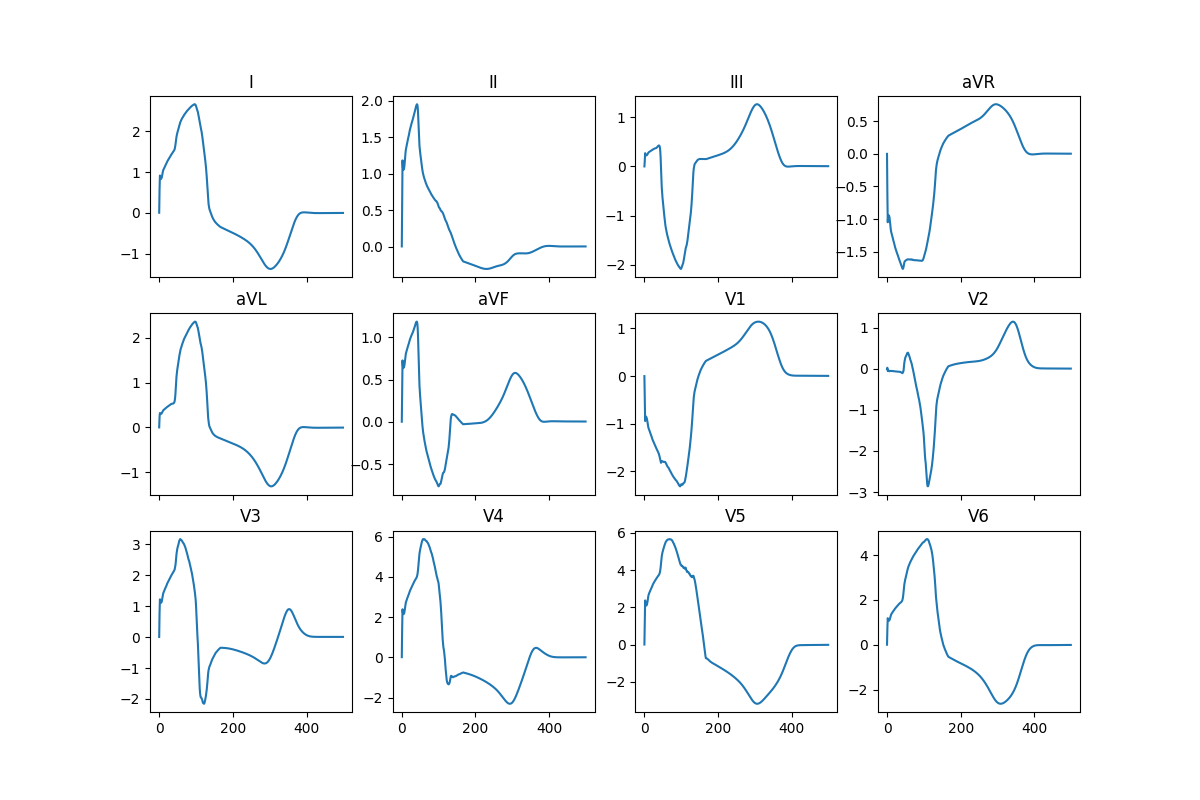
ecg12_lead = beat.ecg.Leads12(**{k: np.array(v) for k, v in ecg_traces.items()})
fig, ax = plt.subplots(3, 4, sharex=True, figsize=(12, 8))
for i, name in enumerate(
    [
        "I",
        "II",
        "III",
        "aVR",
        "aVL",
        "aVF",
        "V1_",
        "V2_",
        "V3_",
        "V4_",
        "V5_",
        "V6_",
    ],
):
    y = getattr(ecg12_lead, name)
    axi = ax.flatten()[i]
    axi.plot(times[: len(y)], y)
    axi.set_title(name.strip("_"))
fig.tight_layout()
fig.savefig(results_folder / "ecg_12_leads.png")

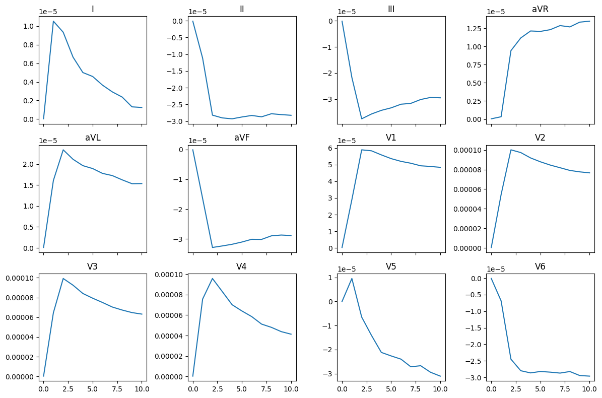
Here are the results from a pre-computed simulation using at characteristic length of the mesh of 0.1 and run it for 500 ms (note that the conduction here seems to be a bit too slow):