Bidomain convergence test#
This demo verifies beat.BidomainModel against a manufactured solution, measuring the
convergence rate of both solved-for fields — the transmembrane potential \(v\) and the
extracellular potential \(u_e\) — in the mesh size \(h\) and in the time step \(\Delta t\). It
closes with the exact collapse onto beat.MonodomainModel that the bidomain model must
exhibit when the two conductivity tensors are proportional.
See the mathematical background page for the bidomain equations and the notation, and the verification demo for the four pitfalls that make convergence measurement harder than it looks. Three of them apply here unchanged, and the fourth is specific to the bidomain system; they are dealt with below as they come up.
The manufactured solution#
The model solves
with insulating boundary conditions. We pick \(v\) and \(u_e\) ourselves and derive the \(I_{stim}\) that makes the first equation exact. The second equation is the awkward one: it has no source term to absorb a mismatch, and adding one is not free either — an elliptic equation with pure Neumann conditions is only solvable when its source is orthogonal to the constants. That is the fourth pitfall, and it has no counterpart in the monodomain case.
We sidestep it entirely. On the unit square, every mode
is an eigenfunction of \(\nabla \cdot (M \nabla \cdot)\) for any constant diagonal \(M\), so the elliptic equation decouples into one scalar equation per mode and we can solve for the amplitudes of \(u_e\) that satisfy it exactly — no source needed. These modes also have vanishing normal derivative on the boundary, so the insulating conditions hold, and vanishing mean, so \(u_e\) meets the model’s zero-mean normalisation.
Two things matter in the choice. The conductivity tensors must not be proportional, and \(v\) must contain more than one mode. Either alone would make \(u_e\) a multiple of \(v\) — the equal anisotropy case — and the coupling between the two equations would go untested while every plot still looked healthy.
import beat
MI = (1.0, 0.4)
ME = (0.3, 1.2)
GAMMA = 0.7
C_M = 1.0
def M_i():
    return ufl.as_matrix([[MI[0], 0.0], [0.0, MI[1]]])
def M_e():
    return ufl.as_matrix([[ME[0], 0.0], [0.0, ME[1]]])
The amplitudes of \(u_e\) that solve the elliptic equation mode by mode. For \(\phi_{11}\) the operators contribute \(4\pi^2(a+b)\) and \(4\pi^2(a+b+c+d)\); for \(\phi_{21}\) the \(x\)-derivative brings a factor of four.
BETA_1 = -(MI[0] + MI[1]) / (MI[0] + MI[1] + ME[0] + ME[1])
BETA_2 = -GAMMA * (4 * MI[0] + MI[1]) / (4 * (MI[0] + ME[0]) + (MI[1] + ME[1]))
def v_exact(x, t):
    return (phi(x, 1, 1) + GAMMA * phi(x, 2, 1)) * ufl.sin(t)
def ue_exact(x, t):
    return (BETA_1 * phi(x, 1, 1) + BETA_2 * phi(x, 2, 1)) * ufl.sin(t)
def l2(expr, mesh):
    form = dolfinx.fem.form(
        ufl.inner(expr, expr) * ufl.dx(domain=mesh, metadata={"quadrature_degree": 8}),
    )
    return np.sqrt(mesh.comm.allreduce(dolfinx.fem.assemble_scalar(form), op=MPI.SUM))
def unit_square(N):
    return dolfinx.mesh.create_unit_square(
        MPI.COMM_WORLD,
        N,
        N,
        dolfinx.mesh.CellType.triangle,
    )
def solve_to(mesh, T, dt, theta=0.5):
    time = dolfinx.fem.Constant(mesh, dolfinx.default_scalar_type(0.0))
    x = ufl.SpatialCoordinate(mesh)
    t = ufl.variable(time)
    model = beat.BidomainModel(
        time=time,
        mesh=mesh,
        M_i=M_i(),
        M_e=M_e(),
        I_s=stimulus(x, t),
        C_m=C_M,
        params=dict(theta=theta),
    )
    model.solve((0.0, T), dt=dt)
    return model
Convergence in space#
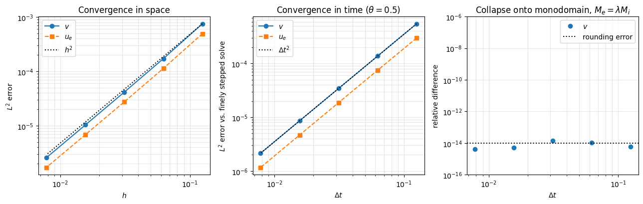
With \(\theta = 0.5\) and a short time interval, the time discretization error is negligible and what is left is the \(P_1\) finite element error, which should fall as \(h^2\) in the \(L^2\) norm for both fields.
The refinement starts at \(N = 8\) rather than \(N = 4\): the second mode fits two full wavelengths across the domain, and a \(4 \times 4\) mesh has not begun to resolve it, so including it would measure the pre-asymptotic regime and understate the rate.
Note also that the exact solution is evaluated at T directly rather than at the UFL
time constant. At \(\theta = 0.5\) that constant sits at \(T - \Delta t / 2\) once the last
step is taken — the second pitfall — and comparing against it would manufacture an error
of order \(\Delta t\) out of nothing.
T_SPACE = 0.01
DT_SPACE = 0.001
NS = [8, 16, 32, 64, 128]
spatial_errors: dict[str, list[float]] = {"v": [], "u_e": []}
hs = []
for N in NS:
    mesh = unit_square(N)
    model = solve_to(mesh, T_SPACE, DT_SPACE)
    x = ufl.SpatialCoordinate(mesh)
    hs.append(1.0 / N)
    spatial_errors["v"].append(l2(model.v - v_exact(x, T_SPACE), mesh))
    spatial_errors["u_e"].append(l2(model.u_e - ue_exact(x, T_SPACE), mesh))
for field, errors in spatial_errors.items():
    rates = [np.log2(e1 / e2) for e1, e2 in zip(errors[:-1], errors[1:])]
    print(f"{field:4s} h-rates: " + ", ".join(f"{r:.2f}" for r in rates))
v    h-rates: 2.13, 2.04, 2.01, 2.00
u_e  h-rates: 2.12, 2.04, 2.01, 2.00
Convergence in time#
Measuring the time discretization error against the exact solution runs straight into the third pitfall: on any mesh this demo can afford, the space discretization error is far larger than the quantity being measured, and the rate flattens out as soon as \(\Delta t\) drops beneath that floor. The monodomain verification demo escapes it by raising the element degree; here we take the other route and compare against a finely stepped solve on the same mesh. The space error is then identical in both solutions and cancels, leaving only the error in time.
\(u_e\) is measured alongside \(v\), and not as an afterthought. The elliptic equation is a constraint rather than an evolution, so the pair is an index-1 differential-algebraic system, and time-stepping schemes can converge more slowly on the algebraic variable than on the differential one. A check that only looked at \(v\) would never see it.
T_TIME = 0.5
N_TIME = 64
LEVELS = [2, 3, 4, 5, 6]
mesh = unit_square(N_TIME)
reference = solve_to(mesh, T_TIME, T_TIME / 2**10)
reference_v = reference.v.copy()
reference_ue = reference.u_e.copy()
temporal_errors: dict[str, list[float]] = {"v": [], "u_e": []}
dts = []
for level in LEVELS:
    dt = T_TIME / 2**level
    model = solve_to(mesh, T_TIME, dt)
    dts.append(dt)
    temporal_errors["v"].append(l2(model.v - reference_v, mesh))
    temporal_errors["u_e"].append(l2(model.u_e - reference_ue, mesh))
for field, errors in temporal_errors.items():
    rates = [np.log2(e1 / e2) for e1, e2 in zip(errors[:-1], errors[1:])]
    print(f"{field:4s} dt-rates: " + ", ".join(f"{r:.2f}" for r in rates))
v    dt-rates: 2.00, 2.00, 2.00, 2.00
u_e  dt-rates: 2.00, 2.00, 2.00, 2.00
The collapse onto the monodomain model#
When \(M_e = \lambda M_i\), the extracellular potential can be eliminated algebraically and the bidomain model becomes the monodomain model with \(M = \frac{\lambda}{1 + \lambda} M_i\). Because \(u_e = -v / (1 + \lambda)\) then lies in the same \(P_1\) space as \(v\), the collapse is exact at the discrete level and not merely in the limit — so the difference between the two models should sit at rounding error for every time step, rather than converging to zero at some rate.
This is a sharper check than it looks. It is the one measurement that pins down the choice of writing both rows of the system at the \(\theta\)-midpoint: impose the elliptic row at the new time instead, and the two models part company at every \(\theta\) below one.
LAMBDA = 2.5
collapse_dts = [T_TIME / 2**level for level in LEVELS]
collapse: list[float] = []
for dt in collapse_dts:
    mesh = unit_square(32)
    time = dolfinx.fem.Constant(mesh, dolfinx.default_scalar_type(0.0))
    x = ufl.SpatialCoordinate(mesh)
    t = ufl.variable(time)
    I_s = stimulus(x, t)

    bidomain = beat.BidomainModel(
        time=time,
        mesh=mesh,
        M_i=M_i(),
        M_e=LAMBDA * M_i(),
        I_s=I_s,
        C_m=C_M,
        params=dict(theta=0.5),
    )
    monodomain = beat.MonodomainModel(
        time=time,
        mesh=mesh,
        M=(LAMBDA / (1.0 + LAMBDA)) * M_i(),
        I_s=I_s,
        C_m=C_M,
        params=dict(theta=0.5),
    )
    bidomain.solve((0.0, T_TIME), dt=dt)
    time.value = 0.0  # type: ignore[assignment]
    monodomain.solve((0.0, T_TIME), dt=dt)

    collapse.append(l2(bidomain.v - monodomain.v, mesh) / l2(monodomain.v, mesh))
print("relative bidomain/monodomain difference: " + ", ".join(f"{c:.2e}" for c in collapse))
relative bidomain/monodomain difference: 5.91e-15, 1.04e-14, 1.43e-14, 5.02e-15, 4.20e-15
The results#
Each panel is log-log, with a dashed reference slope to read the rate against. Markers differ by field so the two curves stay apart without relying on colour.
styles = {"v": ("o", "-"), "u_e": ("s", "--")}

fig, axes = plt.subplots(1, 3, figsize=(13, 4.2))

for field, errors in spatial_errors.items():
    marker, line = styles[field]
    axes[0].loglog(hs, errors, marker=marker, linestyle=line, label=f"${field}$")
axes[0].loglog(
    hs,
    [spatial_errors["v"][0] * (h / hs[0]) ** 2 for h in hs],
    "k:",
    label="$h^2$",
)
axes[0].set_xlabel("$h$")
axes[0].set_ylabel("$L^2$ error")
axes[0].set_title("Convergence in space")

for field, errors in temporal_errors.items():
    marker, line = styles[field]
    axes[1].loglog(dts, errors, marker=marker, linestyle=line, label=f"${field}$")
axes[1].loglog(
    dts,
    [temporal_errors["v"][0] * (dt / dts[0]) ** 2 for dt in dts],
    "k:",
    label=r"$\Delta t^2$",
)
axes[1].set_xlabel(r"$\Delta t$")
axes[1].set_ylabel("$L^2$ error vs. finely stepped solve")
axes[1].set_title(r"Convergence in time ($\theta = 0.5$)")

# No connecting line, and a fixed scale spanning the range the other panels live in:
# these points carry no trend to trace, and letting the axis autoscale to their spread
# would magnify rounding noise into an apparent one.
axes[2].loglog(collapse_dts, collapse, marker="o", linestyle="none", label="$v$")
axes[2].axhline(1e-14, color="k", linestyle=":", label="rounding error")
axes[2].set_ylim(1e-16, 1e-6)
axes[2].set_xlabel(r"$\Delta t$")
axes[2].set_ylabel("relative difference")
axes[2].set_title(r"Collapse onto monodomain, $M_e = \lambda M_i$")

for ax in axes:
    ax.grid(True, which="both", alpha=0.3)
    ax.legend()

fig.tight_layout()
fig.savefig("bidomain_convergence.png", dpi=150)