Monolithic implicit PDE+ODE coupling with dolfinx-external-operator#
The external-operator ODE demo uses beat.ExternalOperatorODESolver
as a drop-in replacement for beat.odesolver.DolfinODESolver inside the same operator-splitting
scheme described in the mathematical background page — same numerics,
different plumbing. This demo goes further: it uses
dolfinx-external-operator’s ability to
supply a derivative for the cell-model right-hand side to solve the PDE and ODE together, in one
fully implicit Newton system, with no operator splitting at all. That eliminates the
operator-splitting error entirely (only the usual temporal/spatial discretization error remains),
something no other solver in this repository can do — MonodomainSplittingSolver is, by
construction, built around alternating PDE and ODE half-steps.
This demo is a prototype, not a new beat API. FEMExternalOperator currently refuses to use a
mixed-space Function as an operand (see below), so the coupled system here is built from N
separate scalar Functions (one per cell-model state) and an N × N block Jacobian, rather than
the flat (num_states, num_points) array DolfinODESolver/ExternalOperatorODESolver use. That
does not scale as cleanly to the 19+ state models used elsewhere in this repository (beat would
need every state’s own block, on top of building and factorizing an N-times-larger coupled linear
system per Newton iteration) — the demo model here is deliberately kept to two states so the pattern
stays readable, but this scalability limitation is real and worth knowing about before reaching for
this pattern on a full-size cell model.
We validate this pattern against an independent, non-FEM reference (a plain scipy.optimize.fsolve
backward-Euler solve, no dolfinx/UFL involved), and then quantify the benefit: for a range of time
steps, we compare the error of this monolithic scheme against MonodomainSplittingSolver with a
realistic Rush–Larsen ODE step (the scheme used throughout the rest of this repository, not a
strawman explicit-Euler comparison), against a well-resolved reference solution.
from pathlib import Path
from mpi4py import MPI
from petsc4py import PETSc
import numpy as np
import basix.ufl
import dolfinx
import dolfinx.fem.petsc
import dolfinx.la.petsc
import ufl
import gotranx
from gotranx.cli.gotran2py import Backend, get_code
import matplotlib.pyplot as plt
import scipy.optimize
import jax
jax.config.update("jax_enable_x64", True)
import jax.numpy as jnp
from dolfinx_external_operator import (
    FEMExternalOperator,
    evaluate_external_operators,
    evaluate_operands,
    replace_external_operators,
)
import beat
The cell model#
We use the same two-state Mitchell–Schaeffer model as the
Irksome demo, generated twice: once through gotranx’s JAX backend
(rhs(t, states, parameters) as a JAX-traceable function, needed for automatic differentiation), and
once as an ordinary NumPy generalized Rush–Larsen scheme (needed for the fair comparison against
MonodomainSplittingSolver, which is how every other tissue demo in this repository steps a cell
model).
ms_ode_code = """
parameters(
    tau_in = 0.3,
    tau_out = 6.0,
    tau_open = 120.0,
    tau_close = 150.0,
    v_gate = 0.13
)
states(
    v = 0.0,
    h = 1.0
)

h_inf = Conditional(Lt(v, v_gate), 1.0, 0.0)
tau_h = Conditional(Lt(v, v_gate), tau_open, tau_close)

dv_dt = h * (v**2 * (1.0 - v)) / tau_in - v / tau_out
dh_dt = (h_inf - h) / tau_h
"""
jax_model_path = Path("ms_jax_monolithic.py")
np_model_path = Path("ms_np_monolithic.py")
if not jax_model_path.is_file() or not np_model_path.is_file():
    ode_path = Path("mitchell_schaeffer_monolithic.ode")
    ode_path.write_text(ms_ode_code)
    ode = gotranx.load_ode(ode_path)
    jax_model_path.write_text(get_code(ode, scheme=None, backend=Backend.jax))
    np_model_path.write_text(
        get_code(ode, scheme=[gotranx.schemes.Scheme.generalized_rush_larsen]),
    )
2026-10-20 17:24:58 [info ] Load ode mitchell_schaeffer_monolithic.ode
2026-10-20 17:24:58 [info ] Num states 2
2026-10-20 17:24:58 [info ] Num parameters 5
import ms_jax_monolithic as ms_jax
import ms_np_monolithic as ms_np
params = np.array(ms_jax.init_parameter_values())
num_states = len(ms_jax.init_state_values())
v_index = ms_jax.state_index("v")
Making the cell model differentiable#
rhs_local is the model’s right-hand side at a single point. jax.vmap extends it to a batch of
points (matching the (num_cells * num_points, num_states) array layout FEMExternalOperator uses),
and jax.jacfwd gives us its exact Jacobian — with no hand-derived derivatives, and no extra effort
even though the model contains a non-smooth Conditional (h_inf, tau_h), which JAX handles like
any other differentiable control flow. This is exactly the pattern used in the
official heat-equation JAX tutorial for
dolfinx-external-operator.
def rhs_local(t, states, parameters):
    return ms_jax.rhs(t, states, parameters)
rhs_vmapped = jax.jit(jax.vmap(rhs_local, in_axes=(None, 0, None)))
jac_vmapped = jax.jit(jax.vmap(jax.jacfwd(rhs_local, argnums=1), in_axes=(None, 0, None)))
A monolithic, fully implicit PDE+ODE Newton problem#
MonolithicCellModelProblem builds the coupled backward-Euler residual
for all states \(v, s\) simultaneously — there is no ODE half-step, no PDE half-step, and no
projection between an ODE space and a PDE space; v and s are solved for at the same time, in the
same Newton system, at the same (new) time level. The rhs_op[i] term for each state is a
FEMExternalOperator wrapping the JAX cell model, and ufl.derivative(F, state, ...) automatically
produces the correct Jacobian contributions through it, including the dqdT/Jacobian branch of
rhs_external, exactly as in dolfinx-external-operator’s own worked examples.
Every Newton iteration needs the external operator’s value and Jacobian refreshed at the current
iterate before the residual/Jacobian are assembled. dolfinx.fem.petsc.NonlinearProblem already
installs a default SNES residual callback that does the right thing for this block (list-of-forms)
problem; we simply wrap it so our constitutive_update runs first, once the current iterate has been
scattered into self.states.
class MonolithicCellModelProblem:
    """A fully implicit, monolithic PDE+ODE Newton problem for an N-state cell model.

    Each state is its own scalar `dolfinx.fem.Function` (not a mixed-space component), since
    `FEMExternalOperator` does not currently support mixed-space operands. State 0 is treated as
    the transmembrane potential $v$: it is the only state that diffuses and receives the
    stimulus. `stim_form` is a callable taking the test function for state 0 and returning the
    full `I_stim * w * d(measure)` contribution to the residual, e.g.
    `lambda w: stim_expr * w * ds(marker)` — passed as a callable (rather than a bare
    expression assumed to integrate over `dx`) specifically so the stimulus's own measure is
    never silently discarded or assumed.
    """

    def __init__(self, mesh, num_states, rhs_fun, jac_fun, params, M, C_m, stim_form, dt):
        V = dolfinx.fem.functionspace(mesh, ("Lagrange", 1))
        self.V = V
        self.states = [dolfinx.fem.Function(V, name=f"state_{i}") for i in range(num_states)]
        self.states_old = [dolfinx.fem.Function(V) for _ in range(num_states)]
        self.num_states = num_states

        w_test = [ufl.TestFunction(V) for _ in range(num_states)]
        d_trial = [ufl.TrialFunction(V) for _ in range(num_states)]

        # The external operator's operand: all states, stacked into one vector-valued expression.
        # (Individually, each self.states[i] lives in a plain, non-mixed space V.)
        V_states = dolfinx.fem.functionspace(
            mesh,
            basix.ufl.element("Lagrange", mesh.basix_cell(), 1, shape=(num_states,)),
        )
        states_expr = ufl.as_vector(self.states)

        def rhs_impl(states_flat):
            states = states_flat.reshape(-1, num_states)
            out = rhs_fun(jnp.array(states), jnp.array(params))
            return np.asarray(out).reshape(-1)

        def jac_impl(states_flat):
            states = states_flat.reshape(-1, num_states)
            out = jac_fun(jnp.array(states), jnp.array(params))
            return np.asarray(out).reshape(-1)

        def rhs_external(derivatives):
            if derivatives == (0,):
                return rhs_impl
            elif derivatives == (1,):
                return jac_impl
            return NotImplementedError

        self.rhs_op = FEMExternalOperator(
            states_expr,
            function_space=V_states,
            external_function=rhs_external,
        )

        dx = ufl.dx
        F = []
        for i in range(num_states):
            coeff = C_m if i == 0 else 1.0
            Fi = coeff * (self.states[i] - self.states_old[i]) / dt * w_test[i] * dx
            Fi -= self.rhs_op[i] * w_test[i] * dx
            if i == 0:
                Fi += ufl.inner(M * ufl.grad(self.states[0]), ufl.grad(w_test[0])) * dx
                # stim_form is the *entire* -I_stim * w_v * d(measure) contribution, built by
                # the caller against w_test[0] — not just an expression, since the stimulus's
                # measure (dx for a volume source, ds(marker) for a boundary one, as here) is
                # significant and must not be silently assumed to be dx.
                Fi -= stim_form(w_test[0])
            F.append(Fi)
        self.F = F

        # N x N block Jacobian: J[i][j] = dF_i/d(state_j). ufl.derivative() picks up the rhs_op
        # Jacobian branch automatically wherever rhs_op[i] depends on state_j.
        self.J = [
            [ufl.derivative(F[i], self.states[j], d_trial[j]) for j in range(num_states)]
            for i in range(num_states)
        ]

        self.F_replaced, self.F_external_operators = [], []
        for Fi in self.F:
            Fi_r, ops = replace_external_operators(Fi)
            self.F_replaced.append(Fi_r)
            self.F_external_operators.extend(ops)
        self.J_replaced, self.J_external_operators = [], []
        for row in self.J:
            row_r = []
            for Jij in row:
                Jij_r, ops = replace_external_operators(Jij)
                row_r.append(Jij_r)
                self.J_external_operators.extend(ops)
            self.J_replaced.append(row_r)

        petsc_options = {
            "snes_type": "newtonls",
            "snes_linesearch_type": "basic",
            "ksp_type": "preonly",
            "pc_type": "lu",
            "snes_atol": 1.0e-9,
            "snes_rtol": 1.0e-9,
            "snes_max_it": 50,
        }
        self.problem = dolfinx.fem.petsc.NonlinearProblem(
            self.F_replaced,
            self.states,
            J=self.J_replaced,
            petsc_options_prefix=f"monolithic_{id(self)}_",
            petsc_options=petsc_options,
        )

        # Wrap the default block-aware residual callback with our external-operator refresh,
        # inserted *after* the current iterate is scattered into self.states (so
        # constitutive_update sees the current Newton iterate) and *before* the residual is
        # assembled (so the assembled residual/Jacobian use the refreshed values).
        _, (orig_func, orig_args, orig_kwargs) = self.problem.solver.getFunction()

        def residual_with_constitutive_update(snes, x, b):
            dolfinx.la.petsc._ghost_update(x, PETSc.InsertMode.INSERT, PETSc.ScatterMode.FORWARD)
            dolfinx.fem.petsc.assign(x, orig_kwargs["u"])
            self.constitutive_update()
            orig_func(snes, x, b, *orig_args, **orig_kwargs)

        self.problem.solver.setFunction(residual_with_constitutive_update, self.problem.b)

    def constitutive_update(self):
        evaluated_operands = evaluate_operands(self.F_external_operators)
        evaluate_external_operators(self.F_external_operators, evaluated_operands)
        evaluate_external_operators(self.J_external_operators, evaluated_operands)

    def step(self):
        self.constitutive_update()
        self.problem.solve()
        for s, s_old in zip(self.states, self.states_old):
            s_old.x.array[:] = s.x.array
        return self.problem.solver.getIterationNumber()
Validating against an independent reference#
Before trusting this on a real mesh, we check it against a completely independent computation: a
plain scipy.optimize.fsolve backward-Euler solve of the same cell model at a single point, with no
dolfinx, UFL or FEMExternalOperator involved at all. We use a state on the nonlinear part of the
model (crossing the Conditional in h_inf/tau_h) so the Jacobian is genuinely exercised.
v0_check, h0_check = 0.9, 0.2
dt_check = 1.0
def backward_euler_residual(states_new, states_old, t, dt, parameters):
    rhs = np.asarray(rhs_local(t, jnp.array(states_new), jnp.array(parameters)))
    return (states_new - states_old) / dt - rhs
check_mesh = dolfinx.mesh.create_unit_square(MPI.COMM_WORLD, 2, 2, dolfinx.mesh.CellType.triangle)
M_zero = dolfinx.fem.Constant(check_mesh, 0.0)
check_problem = MonolithicCellModelProblem(
    check_mesh,
    num_states,
    lambda states, p: rhs_vmapped(0.0, states, p),
    lambda states, p: jac_vmapped(0.0, states, p),
    params,
    M_zero,
    1.0,
    lambda w: 0.0 * w * ufl.dx(domain=check_mesh),  # no stimulus for this check
    dt_check,
)
check_problem.states[0].x.array[:] = v0_check
check_problem.states[1].x.array[:] = h0_check
check_problem.states_old[0].x.array[:] = v0_check
check_problem.states_old[1].x.array[:] = h0_check
check_problem.step()
3
print(f"scipy reference:            v={scipy_ref[0]:.8f}, h={scipy_ref[1]:.8f}")
print(
    f"MonolithicCellModelProblem: v={check_problem.states[0].x.array[0]:.8f}, "
    f"h={check_problem.states[1].x.array[0]:.8f}",
)
max_diff = max(
    np.max(np.abs(check_problem.states[0].x.array - scipy_ref[0])),
    np.max(np.abs(check_problem.states[1].x.array - scipy_ref[1])),
)
print(f"Max abs difference: {max_diff:.3e}")
assert max_diff < 1e-6
scipy reference:            v=0.83639581, h=0.19867550
MonolithicCellModelProblem: v=0.83639581, h=0.19867550
Max abs difference: 2.241e-11
Setting up a small 1D cable#
As in the pacing train and PVC demos, we use a 1D cable rather than a full tissue slab, to keep the runtime of the comparison below small — every implicit timestep here costs a full Newton solve of a coupled, factorized linear system, which is considerably more expensive than either half-step of the default splitting scheme.
comm = MPI.COMM_WORLD
N = 40
L = 1.0
mesh = dolfinx.mesh.create_interval(comm, N, (0.0, L))
M_val = 0.02
C_m = 1.0
T_end = 4.0
stim_amp = 5.0
stim_dur = 1.0
def stim_region(x):
    return x[0] <= 2 * (L / N)
def make_stimulus_tags(mesh):
    tdim = mesh.topology.dim
    facets = dolfinx.mesh.locate_entities_boundary(mesh, tdim - 1, stim_region)
    marker = 1
    tags = dolfinx.mesh.meshtags(
        mesh, tdim - 1, facets, np.full(len(facets), marker, dtype=np.int32),
    )
    return ufl.Measure("ds", domain=mesh, subdomain_data=tags)(marker)
Running the two schemes#
run_split is exactly the existing beat.MonodomainModel + beat.MonodomainSplittingSolver, using
the realistic generalized Rush–Larsen scheme for the ODE step (not a strawman explicit-Euler
comparison). run_monolithic uses MonolithicCellModelProblem above, evaluating the cell model and
the stimulus at the new time level (fully implicit).
def run_split(dt):
    time = dolfinx.fem.Constant(mesh, 0.0)
    ds = make_stimulus_tags(mesh)
    stim_expr = ufl.conditional(ufl.le(time, stim_dur), stim_amp, 0.0)
    I_s = beat.base_model.Stimulus(expr=stim_expr, dZ=ds, marker=1)

    pde = beat.MonodomainModel(time=time, mesh=mesh, M=M_val, I_s=I_s, C_m=C_m)
    V_ode = dolfinx.fem.functionspace(mesh, ("Lagrange", 1))
    N_ode = V_ode.dofmap.index_map.size_local + V_ode.dofmap.index_map.num_ghosts
    init_states = np.zeros((num_states, N_ode))
    init_states.T[:] = ms_jax.init_state_values()

    ode = beat.odesolver.DolfinODESolver(
        v_ode=dolfinx.fem.Function(V_ode),
        v_pde=pde.state,
        fun=ms_np.generalized_rush_larsen,
        init_states=init_states,
        parameters=params,
        num_states=num_states,
        v_index=v_index,
    )
    solver = beat.MonodomainSplittingSolver(pde=pde, ode=ode, theta=1.0)
    t = 0.0
    while t < T_end - 1e-9:
        solver.step((t, t + dt))
        t += dt
    return pde.state.x.array.copy()
def run_monolithic(dt):
    time_c = dolfinx.fem.Constant(mesh, 0.0)
    ds = make_stimulus_tags(mesh)
    stim_expr = ufl.conditional(ufl.le(time_c, stim_dur), stim_amp, 0.0)
    M = dolfinx.fem.Constant(mesh, M_val)

    problem = MonolithicCellModelProblem(
        mesh,
        num_states,
        lambda states, p, _t=time_c: rhs_vmapped(_t.value, states, p),
        lambda states, p, _t=time_c: jac_vmapped(_t.value, states, p),
        params,
        M,
        C_m,
        lambda w: stim_expr * w * ds,
        dt,
    )
    v0, h0 = ms_jax.init_state_values()
    problem.states[0].x.array[:] = v0
    problem.states[1].x.array[:] = h0
    problem.states_old[0].x.array[:] = v0
    problem.states_old[1].x.array[:] = h0

    t = 0.0
    max_its = 0
    while t < T_end - 1e-9:
        time_c.value = t + dt  # fully implicit: stimulus/cell model evaluated at the new time
        max_its = max(max_its, problem.step())
        t += dt
    return problem.states[0].x.array.copy(), max_its
Quantifying the benefit of no splitting error#
We compute a well-resolved reference at a small dt, then compare both schemes against it at a
range of larger, more practical time steps.
dt_ref = 0.01
print("\nComputing reference solution (split scheme, fine dt)...")
v_ref = run_split(dt_ref)
Computing reference solution (split scheme, fine dt)...
dts = [0.5, 0.25, 0.125]
print(f"\n{'dt':<8}{'split (Rush-Larsen) L2 err':<30}{'monolithic L2 err':<20}{'newton its':<12}")
split_errors = []
mono_errors = []
for dt in dts:
    v_split = run_split(dt)
    v_mono, max_its = run_monolithic(dt)
    err_split = float(np.sqrt(np.mean((v_split - v_ref) ** 2)))
    err_mono = float(np.sqrt(np.mean((v_mono - v_ref) ** 2)))
    split_errors.append(err_split)
    mono_errors.append(err_mono)
    print(f"{dt:<8}{err_split:<30.5f}{err_mono:<20.5f}{max_its:<12}")
dt split (Rush-Larsen) L2 err monolithic L2 err newton its
0.5 0.31642 0.11951 14
0.25 0.19209 0.04088 12
0.125 0.12237 0.01244 11
fig, ax = plt.subplots()
ax.loglog(dts, split_errors, "o-", label="MonodomainSplittingSolver (Rush–Larsen)")
ax.loglog(dts, mono_errors, "s-", label="Monolithic implicit (this demo)")
ax.set_xlabel(r"$\Delta t$")
ax.set_ylabel("RMS error vs. fine-$\\Delta t$ reference")
ax.legend()
ax.grid(True, which="both", alpha=0.3)
fig.savefig("monolithic_external_operator_error.png")
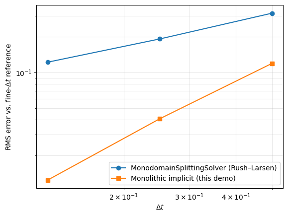
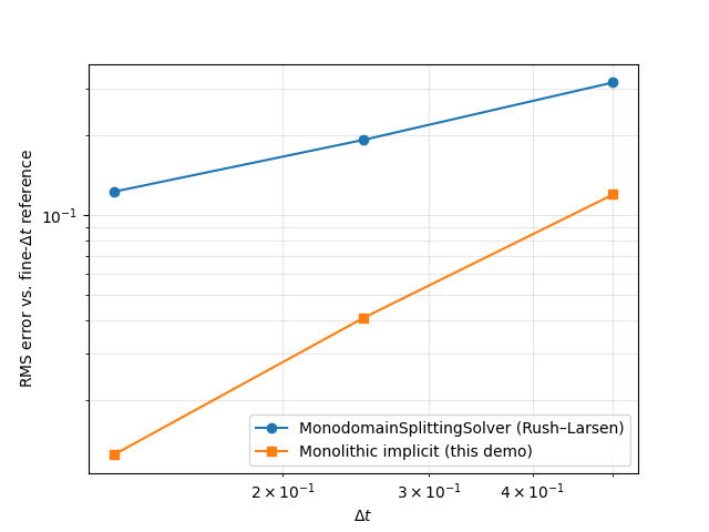
At every timestep tested, removing the operator-splitting error reduces the total error — by roughly 3-10x at these resolutions, though both schemes are still first order overall (backward Euler, and Godunov splitting, are both \(\mathcal{O}(\Delta t)\)), so the gap is in the constant, not the rate. This is the same phenomenon well known for stiff reaction-diffusion systems generally: an explicit or split treatment of the reaction term restricts either the accuracy or the stability of the timestep, while a monolithic implicit treatment does not.
Honest costs#
This comes at a real price, beyond the scalability caveat described at the top of this demo:
MonolithicCellModelProblem.step() performs a full Newton solve — several linear solves of an
num_states-times-larger coupled system — every timestep, compared to one linear PDE solve and one
explicit ODE update for the split scheme. For this two-state model and small cable that cost is
modest; for a full ten Tusscher-sized model it would not be, both because of the block size and
because building the \(19 \times 19\) block Jacobian this way means compiling and assembling 19 diagonal
blocks and up to \(19^2\) (mostly nonzero, since the ionic current couples every gating variable back
into \(v\)) off-diagonal Jacobian blocks. Whether that trade-off is worth it depends on how much the
splitting error actually costs you at the timestep you want to use — which is exactly what the
comparison above lets you check for your own problem.