Fully implicit high-order time stepping with Irksome#
All the other demos in this repository advance the monodomain model with the low-order (first- or second-order accurate) Godunov/Strang splitting scheme described in the mathematical background page: a \(\theta\)-rule for the diffusion PDE step and an explicit or Rush–Larsen scheme for the cell-model ODE step.
beat.IrksomeMonodomainModel and beat.IrksomeODESolver are drop-in alternatives to
beat.MonodomainModel and beat.odesolver.DolfinODESolver/DolfinMultiODESolver that instead use
Irksome to advance the PDE step and/or the ODE step with a
fully implicit Runge–Kutta method, specified as a Butcher tableau (e.g. irksome.BackwardEuler()
for a first-order implicit step, or irksome.GaussLegendre(2) for a fourth-order one). Since they
implement the same pde/ode interfaces as the default solvers, they plug directly into
beat.MonodomainSplittingSolver and can even be mixed with the default solvers (an
IrksomeMonodomainModel PDE step can be paired with a plain DolfinODESolver ODE step, or vice
versa) — see tests/test_monodomain_solver.py::test_irksome_monodomain_splitting_analytic for such
a mix. IrksomeMonodomainModel can also be used entirely on its own (without any splitting or cell
model at all) for a purely implicit, high-order-in-time diffusion equation, as in
tests/test_irksome_monodomain.py.
This is useful when the default low-order splitting is not accurate enough in time, or when the cell-model ODEs are too stiff for the explicit/Rush–Larsen schemes used elsewhere in this repository. The trade-off is that each implicit stage requires solving a (nonlinear, for a nonlinear cell model) system over the whole mesh, which is more expensive per step than the default explicit ODE update.
This demo combines both: a gotranx-generated UFL cell model
(the two-variable Mitchell–Schaeffer model) is solved with IrksomeODESolver, coupled through
beat.MonodomainSplittingSolver (Godunov splitting, \(\theta = 1\)) to an IrksomeMonodomainModel PDE
step, on a domain with a banded, strongly heterogeneous conductivity \(M\). We track when each point
first crosses a voltage threshold to build an activation-time map, which should show fast activation
in the high-conductivity band and progressively slower activation as \(M\) decreases.
Note that irksome is an optional dependency — install it with the irksome extra,
python3 -m pip install fenicsx-beat[irksome].
import beat
from beat.irksome_model import IrksomeMonodomainModel
from beat.irksome_odesolver import IrksomeODESolver
import irksome
import gotranx
import gotranx.cli.gotran2ufl
from gotranx.codegen.python import Format
The cell model#
We define the Mitchell–Schaeffer model — a simple two-variable model (transmembrane potential \(v\)
and a gating variable \(h\)) — directly in gotranx’s declarative .ode language, and use
gotranx.cli.gotran2ufl to translate it into a Python module of UFL expressions (rather than the
plain-numpy expressions used by the other cell-model demos). This UFL form is what
IrksomeODESolver needs, since Irksome differentiates and solves the ODE system as a variational
problem rather than stepping a numpy array by hand.
ms_ode_code = """
parameters(
    tau_in = 0.3,
    tau_out = 6.0,
    tau_open = 120.0,
    tau_close = 150.0,
    v_gate = 0.13
)
states(
    v = 0.0,
    h = 1.0
)

h_inf = Conditional(Lt(v, v_gate), 1.0, 0.0)
tau_h = Conditional(Lt(v, v_gate), tau_open, tau_close)

dv_dt = h * (v**2 * (1.0 - v)) / tau_in - v / tau_out
dh_dt = (h_inf - h) / tau_h
"""
def generate_and_import_cell_model():
    """Generate the UFL Python module from the gotranx string above and import it."""
    ode_filename = Path("mitchell_schaeffer.ode")
    ode_filename.write_text(ms_ode_code)

    gotranx.cli.gotran2ufl.main(
        fname=ode_filename,
        outname="ms_cell_model",
        format=Format.none,  # Disable formatting for speed (or use Format.black)
    )

    # Add local directory to path to import the generated file
    sys.path.insert(0, os.getcwd())
    import ms_cell_model

    return ms_cell_model
Geometry and heterogeneous conductivity#
We solve on a unit square, with the conductivity tensor \(M\) set piecewise-constant in four
horizontal bands, differing by a factor of \(64\) between the fastest (top) and slowest (bottom) band.
A real conductivity tensor would be built with beat.conductivities.define_conductivity_tensor from
physical intra-/extracellular conductivities and a fibre field, as in the other tissue demos; here we
construct it directly to keep the focus on the Irksome time stepping.
def eval_conductivity(x):
    """Evaluate conductivity based on y-coordinate bands."""
    y = x[1]
    conditions = [
        y >= 0.75,
        (y >= 0.50) & (y < 0.75),
        (y >= 0.25) & (y < 0.50),
        y < 0.25,
    ]
    choices = [2.0, 0.5, 0.125, 0.03125]
    return np.select(conditions, choices)
def eval_initial_voltage(x):
    """Stimulate the left edge of the domain."""
    return np.where(x[0] <= 0.05, 1.0, 0.0)
if comm.rank == 0:
    print("Generating UFL Cell Model from gotranx...")
ms_ufl = generate_and_import_cell_model()
Generating UFL Cell Model from gotranx...
2026-10-20 17:19:48 [info     ] Load ode mitchell_schaeffer.ode
2026-10-20 17:19:48 [debug ] Guarded removable singularities assignments=[]
2026-10-20 17:19:48 [info ] Num states 2
2026-10-20 17:19:48 [info ] Num parameters 5
2026-10-20 17:19:48 [debug ] Generating parameter_index with 5 values
2026-10-20 17:19:48 [debug ] Generating state_index with 2 values
2026-10-20 17:19:48 [debug ] Generating monitored_index with 4 values
2026-10-20 17:19:48 [debug ] Generating init_parameter_values with 5 values
2026-10-20 17:19:48 [debug ] Generating init_state_values with 2 values
2026-10-20 17:19:48 [debug ] Generating method 'rhs', with 2 return values.
2026-10-20 17:19:48 [debug ] Generating method 'monitor_values', with 4 return values.
2026-10-20 17:19:48 [info ] Wrote ms_cell_model.py
N = 100
mesh = dolfinx.mesh.create_unit_square(comm, N, N, dolfinx.mesh.CellType.triangle)
time = dolfinx.fem.Constant(mesh, dolfinx.default_scalar_type(0.0))
el_M = basix.ufl.element(family="DG", cell=mesh.basix_cell(), degree=0)
V_M = dolfinx.fem.functionspace(mesh, el_M)
M = dolfinx.fem.Function(V_M, name="Conductivity")
M.interpolate(eval_conductivity)
Initial conditions#
Rather than applying an external stimulus current \(I_{stim}\) (as in most of the other demos), here we trigger the action potential with a localized initial condition: \(v = 1\) (i.e. already fully depolarized) on a thin strip along the left edge of the domain, and the resting state everywhere else. All other state variables (here just the gating variable \(h\)) start at the cell model’s default resting values.
V_ode = dolfinx.fem.functionspace(mesh, ("CG", 1))
v_ode = dolfinx.fem.Function(V_ode, name="V_ode")
# Initialize with -1.0 to denote "not yet activated"
tact_func = dolfinx.fem.Function(V_ode, name="ActivationTime")
tact_func.x.array[:] = -1.0
activation_threshold = 0.02
default_states = ms_ufl.init_state_values()
default_params = ms_ufl.init_parameter_values()
v_idx = ms_ufl.state_index("v")
num_states = len(default_states)
init_states = np.zeros((num_states, v_ode.x.array.size))
for i in range(num_states):
    init_states[i, :] = default_states[i]
v_ode.interpolate(eval_initial_voltage)
init_states[v_idx, :] = v_ode.x.array
Setting up the Irksome PDE and ODE solvers#
We use irksome.BackwardEuler() — a single-stage, first-order implicit Runge–Kutta method — as the
Butcher tableau for both the PDE and ODE steps, matching the (also first-order) Godunov splitting
used below; a higher-order tableau such as irksome.GaussLegendre(2) could be used for either step
without any other changes. We pass no explicit stimulus (I_s=None) since the action potential is
triggered by the initial condition above, and use a block-Jacobi-preconditioned CG solver for the
(here, symmetric positive definite) linear system arising at each implicit stage.
pde_tableau = irksome.BackwardEuler()
params = dict(
    petsc_options={"ksp_type": "cg", "pc_type": "bjacobi", "ksp_rtol": 1e-6},
)
pde = IrksomeMonodomainModel(
    time=time,
    mesh=mesh,
    M=M,
    butcher_tableau=pde_tableau,
    I_s=None,
    params=params,
)
IrksomeODESolver.fun must return UFL expressions for the right-hand side \(f(v, s)\) (unlike the
plain-numpy fun expected by DolfinODESolver), so we wrap the gotranx-generated ms_ufl.rhs to
match the fun(states, t, parameters) signature Irksome expects. We build pde first so that its
state can be passed directly as v_pde here, combining the two into the usual splitting solver —
theta=1.0 selects Godunov splitting, matching the first-order BackwardEuler tableau used for both
sub-steps.
ode_tableau = irksome.BackwardEuler()
def ufl_rhs_wrapper(states, t, p):
    return ms_ufl.rhs(t, states, p)
ode = IrksomeODESolver(
    v_ode=v_ode,
    v_pde=pde.state,
    fun=ufl_rhs_wrapper,
    init_states=init_states,
    butcher_tableau=ode_tableau,
    time=time,
    num_states=num_states,
    v_index=v_idx,
    parameters=default_params,
)
solver = beat.MonodomainSplittingSolver(pde=pde, ode=ode, theta=1.0)
Time stepping#
As in the other tissue demos, we save the transmembrane potential \(v\) to an XDMF file at every step,
and additionally record, for every mesh point, the first time at which \(v\) crosses
activation_threshold — the local activation time.
xdmf = dolfinx.io.XDMFFile(comm, "results_gotranx_irksome.xdmf", "w")
xdmf.write_mesh(mesh)
xdmf.write_function(M, 0.0)
t = 0.0
dt = 0.1
T_end = 2.0
if comm.rank == 0:
    print("Starting fully implicit gotranx+Irksome simulation...")
Starting fully implicit gotranx+Irksome simulation...
while t < T_end - 1e-8:
    if comm.rank == 0:
        print(f"Solving for t = {t:.2f} ms")

    solver.solve((t, t + dt), dt=dt)
    t += dt

    v_arr = pde.state.x.array
    tact_arr = tact_func.x.array
    crossed_threshold_mask = (v_arr >= activation_threshold) & (tact_arr < 0.0)
    tact_arr[crossed_threshold_mask] = t

    pde.state.name = "Voltage"
    xdmf.write_function(pde.state, t)
Solving for t = 0.00 ms
Solving for t = 0.10 ms
Solving for t = 0.20 ms
Solving for t = 0.30 ms
Solving for t = 0.40 ms
Solving for t = 0.50 ms
Solving for t = 0.60 ms
Solving for t = 0.70 ms
Solving for t = 0.80 ms
Solving for t = 0.90 ms
Solving for t = 1.00 ms
Solving for t = 1.10 ms
Solving for t = 1.20 ms
Solving for t = 1.30 ms
Solving for t = 1.40 ms
Solving for t = 1.50 ms
Solving for t = 1.60 ms
Solving for t = 1.70 ms
Solving for t = 1.80 ms
Solving for t = 1.90 ms
Plotting the activation map#
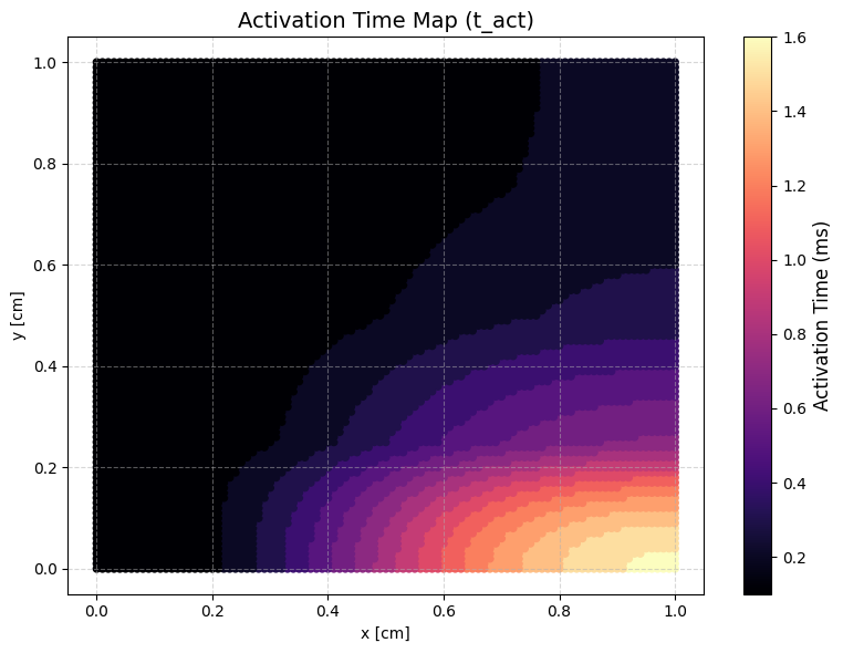
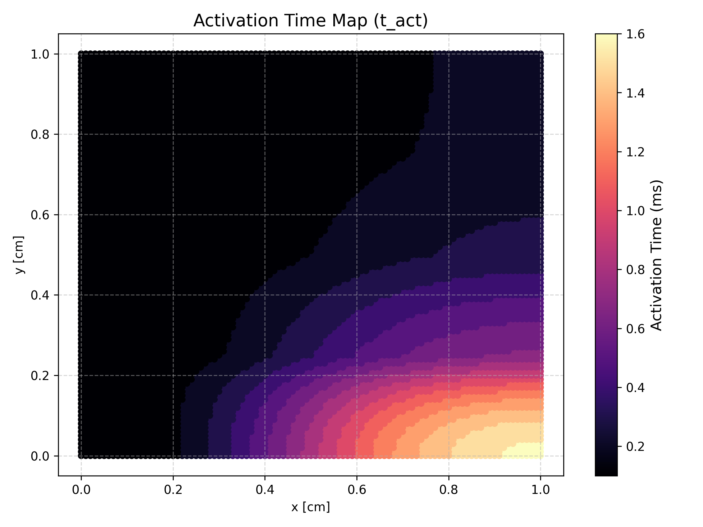
We save the activation-time field to XDMF for visualization in ParaView, and also produce a quick scatter plot directly with matplotlib. The activation time should increase from left to right (away from the initial stimulus) and, within that, increase from top to bottom as the conductivity \(M\) drops by a factor of \(64\) from the fastest to the slowest band.
with dolfinx.io.XDMFFile(comm, "activation_time.xdmf", "w") as xdmf_tact:
    xdmf_tact.write_mesh(mesh)
    xdmf_tact.write_function(tact_func, 0.0)
if comm.rank == 0:
    print("Plotting Activation Times...")
    coords = V_ode.tabulate_dof_coordinates()

    # Mask out any nodes that never activated (if the wave didn't reach them)
    activated_mask = tact_func.x.array >= 0.0

    x = coords[activated_mask, 0]
    y = coords[activated_mask, 1]
    t_acts = tact_func.x.array[activated_mask]

    plt.figure(figsize=(8, 6))
    sc = plt.scatter(x, y, c=t_acts, cmap="magma", s=20)
    cbar = plt.colorbar(sc)
    cbar.set_label("Activation Time (ms)", fontsize=12)
    plt.title("Activation Time Map (t_act)", fontsize=14)
    plt.xlabel("x [cm]")
    plt.ylabel("y [cm]")
    plt.grid(True, linestyle="--", alpha=0.5)
    plt.tight_layout()

    plt.savefig("activation_time_map.png", dpi=300)
    print("Saved 2D activation map to 'activation_time_map.png'.")
Plotting Activation Times...
Saved 2D activation map to 'activation_time_map.png'.
# Prevent MPI hangs during cleanup, since PETSc/MPI resources held by the solver, PDE and ODE
# objects must be released on every rank before the interpreter exits.
comm.Barrier()
del solver
del pde
del ode
comm.Barrier()
gc.collect()
comm.Barrier()