
Forward Euler#
The forward (or explicit) Euler scheme is the simplest method for solving an ODE, and it is the building block for all other schemes in gotranx. In gotranx it is called explicit_euler. The names forward_euler and euler are accepted as aliases by gotranx.schemes.get_scheme().
Mathematics#
Consider the ODE
If we integrate the equation from \(t_n\) to \(t_{n+1} = t_n + \Delta t\) we get
The forward Euler scheme approximates the integral by assuming that the integrand is constant over the step, equal to its value at the start of the step:
Equivalently, (1) follows from replacing the derivative by the forward difference \((y^{n+1} - y^n)/\Delta t\). The scheme is explicit: the new value \(y^{n+1}\) is computed directly from known quantities, and each step costs a single evaluation of \(f\).
Accuracy#
A Taylor expansion of the exact solution gives
so the error made in one step (the local truncation error) is \(\mathcal{O}(\Delta t^2)\). To reach a fixed end time \(T\) we take \(T/\Delta t\) steps, and the errors add up to a global error of \(\mathcal{O}(\Delta t)\). Forward Euler is a first-order method: halving the time step halves the error.
Stability#
To study stability we apply the scheme to the linear test equation
whose exact solution \(y(t) = y_0 e^{\lambda t}\) decays to zero. Forward Euler gives
The numerical solution only decays if \(|1 + \lambda \Delta t| \le 1\), that is if
For a system of ODEs, \(\lambda\) is replaced by the eigenvalues of the Jacobian \(\partial f / \partial y\), and the condition must hold for the eigenvalue with the largest magnitude. In other words, the time step is limited by the fastest time scale of the model, even if that time scale is irrelevant for the solution we are interested in. Problems where this restriction is severe are called stiff. This is the main weakness of forward Euler, and the motivation for the Rush–Larsen family of schemes.
For a thorough treatment of the forward Euler method, its accuracy and its stability, see e.g. Hairer et al. (1993).
Examples#
A linear test problem#
Let us first verify the stability bound (2) on the test equation \(\mathrm{d}y/\mathrm{d}t = \lambda y\) with \(\lambda = -10\). With this \(\lambda\), forward Euler is stable for \(\Delta t \le 0.2\).
import numpy as np
import matplotlib.pyplot as plt
import gotranx

ode = gotranx.load.ode_from_string(
    """
    parameters(lmbda=-10.0)
    states(y=1.0)
    dy_dt = lmbda * y
    """
)
code = gotranx.cli.gotran2py.get_code(
    ode, scheme=[gotranx.schemes.Scheme.explicit_euler]
)
print(code)
2026-10-21 05:31:16 [info ] Num states 1
2026-10-21 05:31:16 [info ] Num parameters 1
import numpy

parameter = {"lmbda": 0}


def parameter_index(name: str) -> int:
    """Return the index of the parameter with the given name

    Arguments
    ---------
    name : str
        The name of the parameter

    Returns
    -------
    int
        The index of the parameter

    Raises
    ------
    KeyError
        If the name is not a valid parameter
    """

    return parameter[name]


state = {"y": 0}


def state_index(name: str) -> int:
    """Return the index of the state with the given name

    Arguments
    ---------
    name : str
        The name of the state

    Returns
    -------
    int
        The index of the state

    Raises
    ------
    KeyError
        If the name is not a valid state
    """

    return state[name]


monitor = {"dy_dt": 0}


def monitor_index(name: str) -> int:
    """Return the index of the monitor with the given name

    Arguments
    ---------
    name : str
        The name of the monitor

    Returns
    -------
    int
        The index of the monitor

    Raises
    ------
    KeyError
        If the name is not a valid monitor
    """

    return monitor[name]


def init_parameter_values(**values):
    """Initialize parameter values"""
    # lmbda=-10.0

    parameters = numpy.array([-10.0], dtype=numpy.float64)

    for key, value in values.items():
        parameters[parameter_index(key)] = value

    return parameters


def init_state_values(**values):
    """Initialize state values"""
    # y=1.0

    states = numpy.array([1.0], dtype=numpy.float64)

    for key, value in values.items():
        states[state_index(key)] = value

    return states


def rhs(t, states, parameters):

    # Assign states
    y = states[0]

    # Assign parameters
    lmbda = parameters[0]

    # Assign expressions

    values = numpy.zeros_like(states, dtype=numpy.float64)
    dy_dt = lmbda * y
    values[0] = dy_dt

    return values


def monitor_values(t, states, parameters):

    # Assign states
    y = states[0]

    # Assign parameters
    lmbda = parameters[0]

    # Assign expressions
    shape = 1 if len(states.shape) == 1 else (1, states.shape[1])
    values = numpy.zeros(shape)
    dy_dt = lmbda * y
    values[0] = dy_dt

    return values


def explicit_euler(states, t, dt, parameters):

    # Assign states
    y = states[0]

    # Assign parameters
    lmbda = parameters[0]

    # Assign expressions

    values = numpy.zeros_like(states, dtype=numpy.float64)
    dy_dt = lmbda * y
    values[0] = dt * dy_dt + y

    return values
The generated function explicit_euler takes one step of (1). We execute the code into a dictionary and use it to solve the problem with three different time steps.
model = {}
exec(code, model)


def solve(step, dt, T, model):
    """Solve the ODE up to time T with the step function `step`."""
    n = int(round(T / dt))
    t = np.linspace(0, T, n + 1)
    y = np.zeros((n + 1, len(model["init_state_values"]())))
    y[0] = model["init_state_values"]()
    p = model["init_parameter_values"]()
    for i in range(n):
        y[i + 1] = step(y[i], t[i], dt, p)
    return t, y


T = 2.0
t_exact = np.linspace(0, T, 500)
fig, ax = plt.subplots()
ax.plot(t_exact, np.exp(-10 * t_exact), "k", label="Exact")
for dt in [0.05, 0.15, 0.21]:
    t, y = solve(model["explicit_euler"], dt, T, model)
    ax.plot(t, y[:, 0], "o-", label=rf"$\Delta t = {dt}$")
ax.set_xlabel("t")
ax.set_ylabel("y")
ax.set_ylim(-1.5, 1.5)
ax.legend()
plt.show()
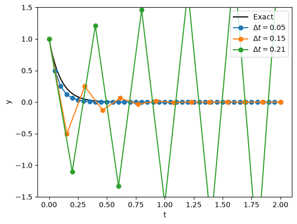
With \(\Delta t = 0.05\) the solution decays monotonically, with \(\Delta t = 0.15\) it oscillates but still decays (\(1 + \lambda \Delta t = -0.5\)), and with \(\Delta t = 0.21\) the oscillations grow (\(1 + \lambda \Delta t = -1.1\)).
When the scheme is stable we can check that it is first order. We compute the error at \(t = 0.5\) for a sequence of time steps, and estimate the convergence rate \(r\) from \(e(\Delta t) \approx C \Delta t^r\) for each pair of consecutive time steps.
T_end = 0.5
dts = np.array([0.01, 0.005, 0.0025, 0.00125, 0.000625])
errors = []
for dt in dts:
    t, y = solve(model["explicit_euler"], dt, T_end, model)
    errors.append(abs(y[-1, 0] - np.exp(-10 * T_end)))
errors = np.array(errors)
rates = np.log(errors[1:] / errors[:-1]) / np.log(dts[1:] / dts[:-1])
print("Errors:", errors)
print("Convergence rates:", np.round(rates, 3))
Errors: [0.00158417 0.00081742 0.00041495 0.00020902 0.0001049 ]
Convergence rates: [0.955 0.978 0.989 0.995]
The convergence rate approaches 1, as expected.
The Hodgkin–Huxley model#
Next we solve the Hodgkin–Huxley model introduced in the overview. We generate code for both the right-hand side and the forward Euler scheme.
ode = gotranx.load_ode("hodgkin_huxley.ode")
code = gotranx.cli.gotran2py.get_code(
    ode, scheme=[gotranx.schemes.Scheme.explicit_euler]
)
hh = {}
exec(code, hh)
V_index = hh["state_index"]("V")
2026-10-21 05:31:16 [info ] Load ode hodgkin_huxley.ode
2026-10-21 05:31:17 [info ] Num states 4
2026-10-21 05:31:17 [info ] Num parameters 10
We first compute a reference solution with an adaptive implicit solver from scipy, using the generated right-hand side rhs.
from scipy.integrate import solve_ivp

T = 20.0  # ms
p = hh["init_parameter_values"]()
t_ref = np.linspace(0, T, 2001)
ref = solve_ivp(
    lambda t, y: hh["rhs"](t, y, p),
    [0, T],
    hh["init_state_values"](),
    method="Radau",
    rtol=1e-10,
    atol=1e-10,
    max_step=0.01,
    t_eval=t_ref,
)
V_ref = ref.y[V_index]
Now we solve the model with forward Euler for a few time steps.
fig, ax = plt.subplots()
ax.plot(t_ref, V_ref, "k", label="Reference")
for dt in [0.01, 0.05, 0.06]:
    with np.errstate(all="ignore"):
        t, y = solve(hh["explicit_euler"], dt, T, hh)
    ax.plot(t, y[:, V_index], "--", label=rf"$\Delta t = {dt}$ ms")
ax.set_xlabel("Time (ms)")
ax.set_ylabel("V (mV)")
ax.set_ylim(-90, 60)
ax.legend()
plt.show()
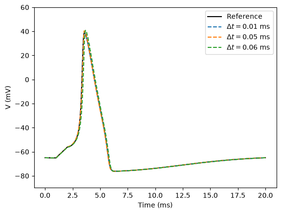
All three solutions are close to the reference. Let us see what happens if we increase the time step slightly more.
for dt in [0.06, 0.08, 0.1]:
    with np.errstate(all="ignore"):
        t, y = solve(hh["explicit_euler"], dt, T, hh)
    V = y[:, V_index]
    if np.all(np.isfinite(V)):
        print(f"dt = {dt} ms: max V = {V.max():.3g} mV")
    else:
        print(f"dt = {dt} ms: the solution blew up")
dt = 0.06 ms: max V = 40.9 mV
dt = 0.08 ms: the solution blew up
dt = 0.1 ms: the solution blew up
The solution blows up. The stiffest equation in this model is the one for the membrane potential. Its diagonal Jacobian entry
reaches about \(-35\ \mathrm{ms}^{-1}\) during the upstroke of the action potential, when the sodium conductance is large. The bound (2) then gives \(\Delta t \lesssim 2/35 \approx 0.057\) ms. The Generalized Rush–Larsen and Hybrid Rush–Larsen pages show how to get rid of this restriction.
From the command line#
The same code can be generated from the command line with
gotranx ode2py hodgkin_huxley.ode --scheme explicit_euler -o hodgkin_huxley.py
and, for example, in C with
gotranx ode2c hodgkin_huxley.ode --scheme explicit_euler -o hodgkin_huxley.h
References#
E. Hairer, S. P. Nørsett and G. Wanner. Solving Ordinary Differential Equations I: Nonstiff Problems. 2nd edition, Springer Series in Computational Mathematics, vol. 8, Springer, 1993. doi:10.1007/978-3-540-78862-1
R. J. Spiteri and R. C. Dean. Stiffness analysis of cardiac electrophysiological models. Annals of Biomedical Engineering, 38(12):3592–3604, 2010. doi:10.1007/s10439-010-0100-9