Hybrid Rush–Larsen#
The hybrid Rush–Larsen scheme combines Forward Euler and Generalized Rush–Larsen. You choose which states are stiff. These are integrated with the exponential Rush–Larsen update, and all the other states are integrated with forward Euler. In gotranx the scheme is called hybrid_rush_larsen, and the stiff states are given with the stiff_states option.
Mathematics#
Let \(S \subseteq \{1, \ldots, N\}\) be the set of stiff states. With \(f_i^n = f_i(t_n, y^n)\) and \(g_i^n = \partial f_i / \partial y_i \, (t_n, y^n)\) as on the Generalized Rush–Larsen page, the hybrid Rush–Larsen scheme is
The other schemes in gotranx are special cases:
Stiff states \(S\) |
Scheme |
|---|---|
none |
|
the gating variables |
the classical Rush–Larsen scheme |
all states |
The same zero-division guard as for generalized Rush–Larsen is used for the stiff states (controlled by delta), and the same common subexpression elimination is applied (controlled by cse).
Why not use generalized Rush–Larsen for everything?#
The exponential update costs one exponential and the evaluation of one diagonal Jacobian entry per state per step. For a model with many states, where only a few of them are stiff, this can be a significant part of the cost of a step. Forward Euler is cheaper, and for a non-stiff state that is integrated with a time step chosen for accuracy, it is often at least as accurate (see the accuracy comparison on the Generalized Rush–Larsen page). The hybrid scheme lets you pay for the exponential update only where it is needed for stability.
Choosing the stiff states#
The scheme is only stable if the forward Euler update is stable for every state not in \(S\). A useful heuristic, based on the stability bound for forward Euler, is to treat state \(i\) as stiff if
where the maximum is taken over a representative solution of the model. This heuristic only looks at the diagonal of the Jacobian and ignores the coupling between the states, so it is not a guarantee. You should always check the stability and accuracy of the result. For a more rigorous analysis based on the eigenvalues of the full Jacobian, see Spiteri and Dean (2010).
Edge cases#
If no stiff states are given, every state is integrated with forward Euler and the scheme is identical to Forward Euler.
If a stiff state has a derivative that does not depend on the state itself (\(g_i \equiv 0\)), the exponential update reduces exactly to forward Euler.
gotranxthen emits the forward Euler update and logs a warning.If a stiff state is not found in the model,
gotranxlogs a warning and ignores it.
Examples#
We continue with the Hodgkin–Huxley model. First we generate the right-hand side and compute a reference solution.
import numpy as np
import matplotlib.pyplot as plt
from scipy.integrate import solve_ivp
import gotranx
from gotranx.schemes import Scheme

ode = gotranx.load_ode("hodgkin_huxley.ode")
code = gotranx.cli.gotran2py.get_code(ode, scheme=[Scheme.explicit_euler])
hh = {}
exec(code, hh)
V_index = hh["state_index"]("V")

T = 20.0  # ms
p = hh["init_parameter_values"]()
t_ref = np.linspace(0, T, 2001)
ref = solve_ivp(
    lambda t, y: hh["rhs"](t, y, p),
    [0, T],
    hh["init_state_values"](),
    method="Radau",
    rtol=1e-10,
    atol=1e-10,
    max_step=0.01,
    t_eval=t_ref,
)
V_ref = ref.y[V_index]
2026-10-21 05:31:27 [info ] Load ode hodgkin_huxley.ode
2026-10-21 05:31:28 [info ] Num states 4
2026-10-21 05:31:28 [info ] Num parameters 10
Finding the stiff states#
To use the heuristic (8) we need \(g_i = \partial f_i / \partial y_i\) along the solution. Here we approximate it with a finite difference of the generated right-hand side. The resulting value \(2 / \max_t |g_i|\) is an estimate of the largest stable forward Euler time step for each state.
states = [s.name for s in ode.states]
max_g = {}
for name in states:
    i = hh["state_index"](name)
    g = []
    for j, t in enumerate(t_ref):
        y = ref.y[:, j]
        eps = 1e-6 * max(1.0, abs(y[i]))
        y_pert = y.copy()
        y_pert[i] += eps
        g.append((hh["rhs"](t, y_pert, p)[i] - hh["rhs"](t, y, p)[i]) / eps)
    max_g[name] = np.max(np.abs(g))

print(f"{'state':>6} {'max |g| (1/ms)':>15} {'2 / max |g| (ms)':>17}")
for name in sorted(states, key=lambda s: -max_g[s]):
    print(f"{name:>6} {max_g[name]:>15.3g} {2 / max_g[name]:>17.3g}")
 state  max |g| (1/ms)  2 / max |g| (ms)
     V            35.5            0.0563
     m            7.91             0.253
     h               1                 2
     n           0.974              2.05
The membrane potential \(V\) is by far the stiffest state, which limits forward Euler (and classical Rush–Larsen, which treats only \(m\), \(h\) and \(n\) exponentially) to \(\Delta t \lesssim 0.056\) ms. The fast sodium activation gate \(m\) comes next, at about \(0.25\) ms, and the slow gates \(h\) and \(n\) only restrict the time step above 2 ms.
According to the heuristic, it is enough to integrate \(V\) exponentially for \(0.056 \lesssim \Delta t \lesssim 0.25\) ms, and \(V\) and \(m\) for larger time steps.
Comparing choices of stiff states#
We generate one step function for each choice of stiff states and compare the root mean square error in \(V\) at a few time steps.
def make_step(stiff_states):
    code = gotranx.cli.gotran2py.get_code(
        ode, scheme=[Scheme.hybrid_rush_larsen], stiff_states=stiff_states
    )
    model = {}
    exec(code, model)
    return model["hybrid_rush_larsen"]


def solve(step, dt):
    n = int(round(T / dt))
    t = np.linspace(0, T, n + 1)
    y = np.zeros((n + 1, len(states)))
    y[0] = hh["init_state_values"]()
    for i in range(n):
        y[i + 1] = step(y[i], t[i], dt, p)
    return t, y


def rms_error(step, dt):
    with np.errstate(all="ignore"):
        t, y = solve(step, dt)
    V = y[:, V_index]
    if not np.all(np.isfinite(V)) or np.abs(V).max() > 1e3:
        return np.nan  # The solution blew up
    return np.sqrt(np.mean((np.interp(t_ref, t, V) - V_ref) ** 2))


choices = {
    "none (forward Euler)": [],
    "m, h, n (Rush-Larsen)": ["m", "h", "n"],
    "V": ["V"],
    "V, m": ["V", "m"],
    "V, m, h, n (GRL)": ["V", "m", "h", "n"],
}
steps = {label: make_step(stiff) for label, stiff in choices.items()}

dts = [0.01, 0.05, 0.1, 0.2, 0.4]
print(f"{'stiff states':>22} " + " ".join(f"{dt:>8}" for dt in dts))
for label, step in steps.items():
    errors = [rms_error(step, dt) for dt in dts]
    print(f"{label:>22} " + " ".join(f"{e:>8.3g}" for e in errors))
          stiff states     0.01     0.05      0.1      0.2      0.4
  none (forward Euler)    0.124    0.653      nan      nan      nan
 m, h, n (Rush-Larsen)    0.834     3.95      nan      nan      nan
                     V    0.612     2.93     5.49     9.75      nan
                  V, m     1.37     6.19     10.9     17.8     31.7
      V, m, h, n (GRL)      1.4      6.4     11.4     18.9     33.6
The results match the heuristic:
With no stiff states, or only the gating variables, the solution blows up (
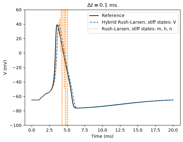
nan) once \(\Delta t\) exceeds the stability limit of the \(V\) equation.Treating only \(V\) as stiff is enough up to \(\Delta t = 0.2\) ms. At \(\Delta t = 0.4\) ms the forward Euler update of \(m\) becomes unstable as well.
Treating \(V\) and \(m\) as stiff gives a stable scheme for all the time steps tested. It needs two exponentials per step, compared with four for generalized Rush–Larsen.
Here is the solution for \(\Delta t = 0.1\) ms with \(V\) as the only stiff state, compared with classical Rush–Larsen:
dt = 0.1
fig, ax = plt.subplots()
ax.plot(t_ref, V_ref, "k", label="Reference")
t, y = solve(steps["V"], dt)
ax.plot(t, y[:, V_index], "--", label="Hybrid Rush-Larsen, stiff states: V")
with np.errstate(all="ignore"):
    t, y = solve(steps["m, h, n (Rush-Larsen)"], dt)
ax.plot(t, y[:, V_index], ":", label="Rush-Larsen, stiff states: m, h, n")
ax.set_ylim(-100, 60)
ax.set_xlabel("Time (ms)")
ax.set_ylabel("V (mV)")
ax.set_title(rf"$\Delta t = {dt}$ ms")
ax.legend()
plt.show()
Generated code#
The generated code only contains the exponential update for the stiff states. Here we generate code with \(V\) and \(m\) as stiff states and print the scheme.
code = gotranx.cli.gotran2py.get_code(
    ode, scheme=[Scheme.hybrid_rush_larsen], stiff_states=["V", "m"]
)
print(code[code.find("def hybrid_rush_larsen"):])
def hybrid_rush_larsen(states, t, dt, parameters):

    # Assign states
    h = states[0]
    m = states[1]
    n = states[2]
    V = states[3]

    # Assign parameters
    Cm = parameters[0]
    E_K = parameters[1]
    E_L = parameters[2]
    E_Na = parameters[3]
    g_K = parameters[4]
    g_L = parameters[5]
    g_Na = parameters[6]
    stim_amp = parameters[7]
    stim_duration = parameters[8]
    stim_start = parameters[9]

    # Assign expressions

    values = numpy.zeros_like(states, dtype=numpy.float64)
    alpha_h = 0.07 * numpy.exp((-(V + 65.0)) / 20.0)
    alpha_m = numpy.where(
        (numpy.abs(V + 40.0) < 0.013894954943731372),
        2.710505431213761e-20 * V**3
        + 0.0008333333333333376 * V**2
        + 0.11666666666666689 * V
        + 4.3333333333333375,
        (0.1 * (V + 40.0)) / (1.0 - numpy.exp((-(V + 40.0)) / 10.0)),
    )
    alpha_n = numpy.where(
        (numpy.abs(V + 55.0) < 0.013894954943731372),
        2.7105054312137612e-21 * V**3
        + 8.333333333333389e-05 * V**2
        + 0.014166666666666704 * V
        + 0.6270833333333342,
        (0.01 * (V + 55.0)) / (1.0 - numpy.exp((-(V + 55.0)) / 10.0)),
    )
    beta_h = 1.0 / (numpy.exp((-(V + 35.0)) / 10.0) + 1.0)
    beta_m = 4.0 * numpy.exp((-(V + 65.0)) / 18.0)
    beta_n = 0.125 * numpy.exp((-(V + 65.0)) / 80.0)
    i_K = (g_K * n**4) * (-E_K + V)
    i_L = g_L * (-E_L + V)
    i_Na = (h * (g_Na * m**3)) * (-E_Na + V)
    i_stim = numpy.where(
        numpy.logical_and((stim_start <= t), (t <= stim_duration + stim_start)),
        stim_amp,
        0.0,
    )
    dh_dt = alpha_h * (1 - h) - beta_h * h
    values[0] = dh_dt * dt + h
    dm_dt = alpha_m * (1 - m) - beta_m * m
    dm_dt_linearized = -alpha_m - beta_m
    values[1] = m + numpy.where(
        numpy.logical_or((dm_dt_linearized > 1e-08), (dm_dt_linearized < -1e-08)),
        dm_dt * (numpy.exp(dm_dt_linearized * dt) - 1) / dm_dt_linearized,
        dm_dt * dt,
    )
    dn_dt = alpha_n * (1 - n) - beta_n * n
    values[2] = dn_dt * dt + n
    dV_dt = (-i_L + (-i_K + (-i_Na + i_stim))) / Cm
    dV_dt_linearized = -(g_K * n**4 + g_L + g_Na * h * m**3) / Cm
    values[3] = V + numpy.where(
        numpy.logical_or((dV_dt_linearized > 1e-08), (dV_dt_linearized < -1e-08)),
        dV_dt * (numpy.exp(dV_dt_linearized * dt) - 1) / dV_dt_linearized,
        dV_dt * dt,
    )

    return values
The gates \(h\) and \(n\) are updated with forward Euler (values[0] and values[2]), while \(m\) and \(V\) get the exponential update with a _linearized variable. The numpy.where expressions in alpha_m and alpha_n are not part of the scheme. They come from gotranx removing the removable singularities at \(V = -40\) mV and \(V = -55\) mV when the model is loaded.
From the command line and the configuration file#
On the command line the stiff states are given with -s or --stiff-states, once for each state:
gotranx ode2py hodgkin_huxley.ode --scheme hybrid_rush_larsen -s V -s m -o hodgkin_huxley.py
In a configuration file they are given as a list:
[tool.gotranx]
scheme = ["hybrid_rush_larsen"]
stiff_states = ["V", "m"]
References#
R. J. Spiteri and R. C. Dean. Stiffness analysis of cardiac electrophysiological models. Annals of Biomedical Engineering, 38(12):3592–3604, 2010. doi:10.1007/s10439-010-0100-9
M. E. Marsh, S. Torabi Ziaratgahi and R. J. Spiteri. The secrets to the success of the Rush–Larsen method and its generalizations. IEEE Transactions on Biomedical Engineering, 59(9):2506–2515, 2012. doi:10.1109/TBME.2012.2205575
S. Rush and H. Larsen. A practical algorithm for solving dynamic membrane equations. IEEE Transactions on Biomedical Engineering, BME-25(4):389–392, 1978. doi:10.1109/TBME.1978.326270
J. Sundnes, R. Artebrant, O. Skavhaug and A. Tveito. A second-order algorithm for solving dynamic cell membrane equations. IEEE Transactions on Biomedical Engineering, 56(10):2546–2548, 2009. doi:10.1109/TBME.2009.2014739