Generalized Rush–Larsen#
The classical Rush–Larsen scheme only works for gating variables, whose equations are linear in the gate. The generalized Rush–Larsen (GRL) scheme extends the idea to every state of the model by linearizing each equation around the current solution, see Sundnes et al. (2009) and Perego and Veneziani (2009). In gotranx the scheme is called generalized_rush_larsen. It is the scheme used in most of the examples in this documentation.
Mathematics#
Derivation#
Consider the system
Over the step from \(t_n\) to \(t_{n+1}\), we replace each right-hand side \(f_i\) by its linearization around \(y^n\) with respect to its own state \(y_i\) only, keeping \(t\) and all the other states fixed:
The numbers \(g_i^n\) are the diagonal entries of the Jacobian \(\partial f / \partial y\). The result is \(N\) decoupled, linear, scalar ODEs with constant coefficients,
which we can solve exactly. Evaluating the solution at \(t_{n+1}\) gives the generalized Rush–Larsen scheme
If we introduce the function \(\varphi_1(z) = (e^z - 1)/z\), the scheme can be written as
Compared with Forward Euler we see that each component of the update is scaled by \(\varphi_1(g_i^n \Delta t)\). This is the exponential Euler method, with the full Jacobian replaced by its diagonal, see Hochbruck and Ostermann (2010) for an overview of exponential integrators.
Properties#
Exact for linear scalar equations. For \(\mathrm{d}y/\mathrm{d}t = \lambda y\) the scheme gives \(y^{n+1} = e^{\lambda \Delta t} y^n\), which is the exact solution. There is no stability restriction on \(\Delta t\) for this test equation, unlike the bound \(\Delta t \le 2/|\lambda|\) for forward Euler.
Reduces to Rush–Larsen for gating variables. For a gating equation \(\mathrm{d}y/\mathrm{d}t = (y_\infty - y)/\tau\) we have \(g = -1/\tau\), and (6) is the classical Rush–Larsen update (see Rush–Larsen).
Reduces to forward Euler when \(g_i = 0\). Since \(\varphi_1(z) \to 1\) as \(z \to 0\), a state whose derivative does not depend on the state itself is updated with forward Euler. This is the exact limit of (6), not an approximation.
First order. The scheme is first-order accurate. A second-order variant (GRL2) is described by Sundnes et al. (2009). It is not available in
gotranx.Cost. Each step needs the right-hand side, the diagonal Jacobian entries and one exponential per state.
Implementation details#
The diagonal Jacobian. gotranx computes \(g_i = \partial f_i / \partial y_i\) symbolically with sympy when the code is generated, see gotranx.linearization.diagonal_jacobian(). The derivative is taken through the intermediate expressions in the model. For example, if dV_dt depends on an intermediate i_Na, which depends on V, that dependence is included. The result therefore does not depend on how the model author split the equations into intermediates. In the generated code \(g_i\) is stored in a variable called d<state>_dt_linearized.
Division by zero. The quotient \(f_i / g_i\) in (6) is not defined when \(g_i = 0\). If gotranx can prove that \(g_i\) is identically zero, it emits the forward Euler update for that state. If it can prove that \(g_i\) is never zero, it emits (6) directly. Otherwise it emits a guard:
The tolerance \(\delta\) defaults to \(10^{-8}\) and can be changed with the --delta flag on the command line, the delta key in the configuration file, or the delta argument in Python.
Common subexpressions. The linearized expressions often share subexpressions, both with each other and with the right-hand side. By default gotranx factors these out with a common subexpression elimination pass into temporaries named _linearization_temp_<k>. Pass --no-cse (or cse=False in Python) to inline them instead, which can save memory in the vectorized numpy backend.
Examples#
Generated code#
To see what the generated code looks like, we use a small model with one gating variable and a nonlinear equation for \(V\).
import numpy as np
import matplotlib.pyplot as plt
import gotranx
from gotranx.schemes import Scheme

ode = gotranx.load.ode_from_string(
    """
    parameters(g=2.0, E=1.0, a=0.5, b=0.1)
    states(V=0.0, w=0.0)
    dV_dt = -g * w * (V - E) - V**3
    dw_dt = a * (1 - w) - b * w
    """
)
code = gotranx.cli.gotran2py.get_code(
    ode, scheme=[Scheme.generalized_rush_larsen]
)
print(code[code.find("def generalized_rush_larsen"):])
2026-10-21 05:31:20 [info ] Num states 2
2026-10-21 05:31:20 [info ] Num parameters 4
def generalized_rush_larsen(states, t, dt, parameters):

    # Assign states
    V = states[0]
    w = states[1]

    # Assign parameters
    E = parameters[0]
    a = parameters[1]
    b = parameters[2]
    g = parameters[3]

    # Assign expressions

    values = numpy.zeros_like(states, dtype=numpy.float64)
    dV_dt = -(V**3) + ((-g) * w) * (-E + V)
    dV_dt_linearized = -3 * V**2 - g * w
    values[0] = V + numpy.where(
        numpy.logical_or((dV_dt_linearized > 1e-08), (dV_dt_linearized < -1e-08)),
        dV_dt * (numpy.exp(dV_dt_linearized * dt) - 1) / dV_dt_linearized,
        dV_dt * dt,
    )
    dw_dt = a * (1 - w) - b * w
    dw_dt_linearized = -a - b
    values[1] = w + numpy.where(
        numpy.logical_or((dw_dt_linearized > 1e-08), (dw_dt_linearized < -1e-08)),
        dw_dt * (numpy.exp(dt * dw_dt_linearized) - 1) / dw_dt_linearized,
        dt * dw_dt,
    )

    return values
dV_dt_linearized is \(\partial f_V / \partial V = -g w - 3V^2\), which can be zero, so the update for V is guarded. dw_dt_linearized is \(-(a + b)\), which gotranx cannot prove to be non-zero because the parameters can take any value, so it is also guarded.
We can also compute the diagonal Jacobian directly from Python. For the Hodgkin–Huxley model we get
from gotranx.linearization import diagonal_jacobian

hh_ode = gotranx.load_ode("hodgkin_huxley.ode")
for state, g in diagonal_jacobian(hh_ode).items():
    print(f"d(d{state}_dt)/d{state} = {g}")
2026-10-21 05:31:21 [info ] Load ode hodgkin_huxley.ode
2026-10-21 05:31:22 [info ] Num states 4
2026-10-21 05:31:22 [info ] Num parameters 10
d(dV_dt)/dV = -g_K*n**4/Cm - g_L/Cm - g_Na*h*m**3/Cm
d(dh_dt)/dh = -alpha_h - beta_h
d(dm_dt)/dm = -alpha_m - beta_m
d(dn_dt)/dn = -alpha_n - beta_n
The Hodgkin–Huxley model#
On the Forward Euler and Rush–Larsen pages we saw that both schemes blow up for the Hodgkin–Huxley model when \(\Delta t = 0.1\) ms, because the equation for \(V\) is stiff. Let us try the generalized Rush–Larsen scheme.
from scipy.integrate import solve_ivp

code = gotranx.cli.gotran2py.get_code(
    hh_ode, scheme=[Scheme.explicit_euler, Scheme.generalized_rush_larsen]
)
hh = {}
exec(code, hh)
V_index = hh["state_index"]("V")


def solve(step, dt, T, model):
    """Solve the ODE up to time T with the step function `step`."""
    n = int(round(T / dt))
    t = np.linspace(0, T, n + 1)
    y = np.zeros((n + 1, len(model["init_state_values"]())))
    y[0] = model["init_state_values"]()
    p = model["init_parameter_values"]()
    for i in range(n):
        y[i + 1] = step(y[i], t[i], dt, p)
    return t, y


# Reference solution
T = 20.0  # ms
p = hh["init_parameter_values"]()
t_ref = np.linspace(0, T, 2001)
ref = solve_ivp(
    lambda t, y: hh["rhs"](t, y, p),
    [0, T],
    hh["init_state_values"](),
    method="Radau",
    rtol=1e-10,
    atol=1e-10,
    max_step=0.01,
    t_eval=t_ref,
)
V_ref = ref.y[V_index]

fig, ax = plt.subplots()
ax.plot(t_ref, V_ref, "k", label="Reference")
for dt in [0.01, 0.1, 0.25]:
    t, y = solve(hh["generalized_rush_larsen"], dt, T, hh)
    ax.plot(t, y[:, V_index], "--", label=rf"GRL, $\Delta t = {dt}$ ms")
ax.set_xlabel("Time (ms)")
ax.set_ylabel("V (mV)")
ax.legend()
plt.show()
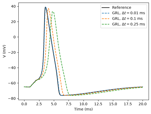
The scheme stays stable with time steps that are several times larger than the forward Euler limit. With \(\Delta t = 0.25\) ms the action potential is clearly delayed, but the solution remains bounded and qualitatively correct.
Accuracy#
A stable scheme is not necessarily an accurate one. Let us compare the root mean square error in \(V\) for forward Euler and generalized Rush–Larsen.
def rms_error(step, dt):
    with np.errstate(all="ignore"):
        t, y = solve(step, dt, T, hh)
    V = y[:, V_index]
    if not np.all(np.isfinite(V)) or np.abs(V).max() > 1e3:
        return np.nan  # The solution blew up
    return np.sqrt(np.mean((np.interp(t_ref, t, V) - V_ref) ** 2))


dts = [0.0025, 0.005, 0.01, 0.02, 0.04, 0.08, 0.16]
print(f"{'dt (ms)':>8} {'Forward Euler':>14} {'GRL':>8}")
for dt in dts:
    fe = rms_error(hh["explicit_euler"], dt)
    grl = rms_error(hh["generalized_rush_larsen"], dt)
    print(f"{dt:>8} {fe:>14.3g} {grl:>8.3g}")
dt (ms) Forward Euler GRL
  0.0025         0.0306    0.355
   0.005         0.0615    0.708
    0.01          0.124      1.4
    0.02          0.251     2.75
    0.04          0.516     5.25
    0.08            nan     12.4
    0.16            nan     26.6
Both schemes are first order: the error is halved when the time step is halved. For this model, forward Euler is actually more accurate than generalized Rush–Larsen for a given time step, as long as it is stable. The benefit of generalized Rush–Larsen is that it stays stable for larger time steps (nan means that forward Euler blew up). In practice the time step is usually limited by accuracy, so you should always check that your results do not change when \(\Delta t\) is reduced. For models with very fast gating dynamics, such as many cardiac cell models, the stability of generalized Rush–Larsen is often what makes it the better choice.
From the command line#
gotranx ode2py hodgkin_huxley.ode --scheme generalized_rush_larsen -o hodgkin_huxley.py
gotranx ode2c hodgkin_huxley.ode --scheme generalized_rush_larsen --delta 1e-10 -o hodgkin_huxley.h
References#
J. Sundnes, R. Artebrant, O. Skavhaug and A. Tveito. A second-order algorithm for solving dynamic cell membrane equations. IEEE Transactions on Biomedical Engineering, 56(10):2546–2548, 2009. doi:10.1109/TBME.2009.2014739
M. Perego and A. Veneziani. An efficient generalization of the Rush–Larsen method for solving electro-physiology membrane equations. Electronic Transactions on Numerical Analysis, 35:234–256, 2009. ETNA vol. 35
M. E. Marsh, S. Torabi Ziaratgahi and R. J. Spiteri. The secrets to the success of the Rush–Larsen method and its generalizations. IEEE Transactions on Biomedical Engineering, 59(9):2506–2515, 2012. doi:10.1109/TBME.2012.2205575
M. Hochbruck and A. Ostermann. Exponential integrators. Acta Numerica, 19:209–286, 2010. doi:10.1017/S0962492910000048
S. Rush and H. Larsen. A practical algorithm for solving dynamic membrane equations. IEEE Transactions on Biomedical Engineering, BME-25(4):389–392, 1978. doi:10.1109/TBME.1978.326270