
Rush–Larsen#
The Rush–Larsen scheme was introduced by Rush and Larsen (1978) for the Hodgkin–Huxley type models used in electrophysiology. It is still one of the most widely used schemes for cardiac cell models. The idea is to integrate the gating variables with an exponential update that is exact if the membrane potential is held fixed, and all other variables with Forward Euler.
Mathematics#
Gating variables#
In a Hodgkin–Huxley type model, the ion channels are controlled by gating variables \(y \in [0, 1]\) that satisfy equations of the form
where \(\alpha(V)\) and \(\beta(V)\) are voltage dependent rates, and
are the steady state value and the time constant of the gate. Some of these time constants are very small, which makes the model stiff. In the Hodgkin–Huxley model, for example, the sodium activation gate \(m\) has \(\tau_m\) well below one millisecond.
The scheme#
The key observation is that (3) is linear in \(y\). If we assume that the membrane potential \(V\), and hence \(y_\infty\) and \(\tau\), is constant over a time step, the equation can be solved exactly:
All the other states (the membrane potential and, in more detailed models, ion concentrations) are updated with forward Euler,
Properties#
Stability for the gating variables. For a fixed \(V\), the update (4) is the exact solution of (3), so it is stable for any time step. The fast gates no longer restrict \(\Delta t\).
Bounded gates. Since \(0 < e^{-\Delta t / \tau} < 1\), the new value \(y^{n+1}\) is a convex combination of \(y^n\) and \(y_\infty \in [0, 1]\). If \(y^n \in [0, 1]\), then \(y^{n+1} \in [0, 1]\) for every \(\Delta t\). Forward Euler can overshoot when \(\Delta t > \tau\).
First order. Freezing \(V\) over the step introduces an \(\mathcal{O}(\Delta t^2)\) local error, so the scheme is first-order accurate, like forward Euler.
The other states are still explicit. The membrane potential is updated with forward Euler, so the stability restriction from the \(V\) equation remains. See Generalized Rush–Larsen for a scheme that also removes this restriction.
The Rush–Larsen scheme can be seen as a simple exponential integrator (Hochbruck and Ostermann, 2010). Marsh et al. (2012) analyze why the method and its generalizations work so well for cardiac cell models.
The form used in gotranx#
gotranx does not look for \(\alpha\), \(\beta\), \(y_\infty\) or \(\tau\) in your model. Instead it writes the update for a state \(y_i\) in the general form
where \(g_i\) is computed symbolically. For the gating equation (3) we have \(f = (y_\infty - y)/\tau\) and \(g = -1/\tau\), so
which is exactly (4). The advantage of (5) is that it does not require the equations to be written in a specific form, and it can be applied to any state. This is the starting point for the Generalized Rush–Larsen and Hybrid Rush–Larsen schemes.
Rush–Larsen in gotranx#
There is no separate rush_larsen scheme in gotranx. The classical Rush–Larsen scheme is the Hybrid Rush–Larsen scheme with the gating variables as the stiff states:
gotranx ode2py hodgkin_huxley.ode --scheme hybrid_rush_larsen -s m -s h -s n -o hodgkin_huxley.py
In Python, gotranx.schemes.get_scheme() also accepts "rush_larsen" as an alias for "hybrid_rush_larsen".
Examples#
The update is exact for a gating variable#
We can use sympy to verify that the general form (5) reduces to the classical Rush–Larsen update (4) for a gating variable.
import sympy

y, alpha, beta, dt = sympy.symbols("y alpha beta Delta_t", positive=True)
f = alpha * (1 - y) - beta * y
g = sympy.diff(f, y)
general = y + f / g * (sympy.exp(g * dt) - 1)

y_inf = alpha / (alpha + beta)
tau = 1 / (alpha + beta)
classical = y_inf + (y - y_inf) * sympy.exp(-dt / tau)

print("g =", g)
print("Difference:", sympy.simplify(general - classical))
g = -alpha - beta
Difference: 0
A single gate at a fixed voltage#
Let us look at the sodium activation gate \(m\) of the Hodgkin–Huxley model with the membrane potential clamped at \(V = 0\) mV. Then \(\tau_m \approx 0.24\) ms and \(m_\infty \approx 0.97\). We generate code for both forward Euler and the hybrid Rush–Larsen scheme with \(m\) as the stiff state.
import numpy as np
import matplotlib.pyplot as plt
import gotranx
from gotranx.schemes import Scheme

ode = gotranx.load.ode_from_string(
    """
    parameters(V=0.0)
    states(m=0.05)
    alpha_m = 0.1 * (V + 40.0) / (1.0 - exp(-(V + 40.0) / 10.0))
    beta_m = 4.0 * exp(-(V + 65.0) / 18.0)
    dm_dt = alpha_m * (1 - m) - beta_m * m
    """
)
code = gotranx.cli.gotran2py.get_code(
    ode,
    scheme=[Scheme.explicit_euler, Scheme.hybrid_rush_larsen],
    stiff_states=["m"],
)
gate = {}
exec(code, gate)
print(code[code.find("def hybrid_rush_larsen"):])
2026-10-21 05:31:34 [info ] Num states 1
2026-10-21 05:31:34 [info ] Num parameters 1
def hybrid_rush_larsen(states, t, dt, parameters):

    # Assign states
    m = states[0]

    # Assign parameters
    V = parameters[0]

    # Assign expressions

    values = numpy.zeros_like(states, dtype=numpy.float64)
    alpha_m = (0.1 * (V + 40.0)) / (1.0 - numpy.exp((-(V + 40.0)) / 10.0))
    beta_m = 4.0 * numpy.exp((-(V + 65.0)) / 18.0)
    dm_dt = alpha_m * (1 - m) - beta_m * m
    dm_dt_linearized = -alpha_m - beta_m
    values[0] = m + numpy.where(
        numpy.logical_or((dm_dt_linearized > 1e-08), (dm_dt_linearized < -1e-08)),
        dm_dt * (numpy.exp(dm_dt_linearized * dt) - 1) / dm_dt_linearized,
        dm_dt * dt,
    )

    return values
The variable dm_dt_linearized is \(g = \partial f / \partial m = -(\alpha_m + \beta_m) = -1/\tau_m\). The numpy.where guards against division by zero (see Generalized Rush–Larsen). We solve the problem with a time step that is about twice the time constant.
def solve(step, dt, T, model):
    """Solve the ODE up to time T with the step function `step`."""
    n = int(round(T / dt))
    t = np.linspace(0, T, n + 1)
    y = np.zeros((n + 1, len(model["init_state_values"]())))
    y[0] = model["init_state_values"]()
    p = model["init_parameter_values"]()
    for i in range(n):
        y[i + 1] = step(y[i], t[i], dt, p)
    return t, y


alpha_m = 0.1 * 40.0 / (1.0 - np.exp(-4.0))
beta_m = 4.0 * np.exp(-65.0 / 18.0)
m_inf, tau_m = alpha_m / (alpha_m + beta_m), 1 / (alpha_m + beta_m)
print(f"m_inf = {m_inf:.3f}, tau_m = {tau_m:.3f} ms")

T = 3.0
dt = 0.5
t_exact = np.linspace(0, T, 300)
m_exact = m_inf + (0.05 - m_inf) * np.exp(-t_exact / tau_m)

fig, ax = plt.subplots()
ax.plot(t_exact, m_exact, "k", label="Exact")
t, m = solve(gate["explicit_euler"], dt, T, gate)
ax.plot(t, m, "o--", label="Forward Euler")
t, m = solve(gate["hybrid_rush_larsen"], dt, T, gate)
ax.plot(t, m, "s--", label="Rush–Larsen")
ax.axhline(1.0, color="gray", lw=0.5)
ax.set_xlabel("Time (ms)")
ax.set_ylabel("m")
ax.set_title(rf"$\Delta t = {dt}$ ms")
ax.legend()
plt.show()
m_inf = 0.974, tau_m = 0.239 ms
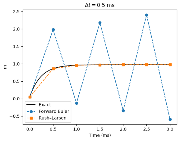
Forward Euler overshoots \(m = 1\) and the oscillations grow, because \(\Delta t > 2 \tau_m\). The Rush–Larsen values coincide with the exact solution at every time step, since the rates are constant in this example.
The Hodgkin–Huxley model#
Now we apply the scheme to the full Hodgkin–Huxley model, with the three gating variables as stiff states and the membrane potential integrated with forward Euler.
from scipy.integrate import solve_ivp

ode = gotranx.load_ode("hodgkin_huxley.ode")
code = gotranx.cli.gotran2py.get_code(
    ode,
    scheme=[Scheme.explicit_euler, Scheme.hybrid_rush_larsen],
    stiff_states=["m", "h", "n"],
)
hh = {}
exec(code, hh)
V_index = hh["state_index"]("V")

# Reference solution
T = 20.0  # ms
p = hh["init_parameter_values"]()
t_ref = np.linspace(0, T, 2001)
ref = solve_ivp(
    lambda t, y: hh["rhs"](t, y, p),
    [0, T],
    hh["init_state_values"](),
    method="Radau",
    rtol=1e-10,
    atol=1e-10,
    max_step=0.01,
    t_eval=t_ref,
)

fig, ax = plt.subplots()
ax.plot(t_ref, ref.y[V_index], "k", label="Reference")
for dt in [0.01, 0.05]:
    t, y = solve(hh["hybrid_rush_larsen"], dt, T, hh)
    ax.plot(t, y[:, V_index], "--", label=rf"Rush–Larsen, $\Delta t = {dt}$ ms")
ax.set_xlabel("Time (ms)")
ax.set_ylabel("V (mV)")
ax.legend()
plt.show()
2026-10-21 05:31:34 [info ] Load ode hodgkin_huxley.ode
2026-10-21 05:31:36 [info ] Num states 4
2026-10-21 05:31:36 [info ] Num parameters 10
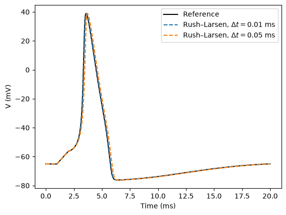
The scheme converges to the reference solution as \(\Delta t\) decreases. However, it does not allow a larger time step than forward Euler for this model:
for dt in [0.06, 0.08, 0.1]:
    for name in ["explicit_euler", "hybrid_rush_larsen"]:
        with np.errstate(all="ignore"):
            t, y = solve(hh[name], dt, T, hh)
        V = y[:, V_index]
        if np.all(np.isfinite(V)):
            print(f"{name:>20}, dt = {dt} ms: max V = {V.max():.3g} mV")
        else:
            print(f"{name:>20}, dt = {dt} ms: the solution blew up")
      explicit_euler, dt = 0.06 ms: max V = 40.9 mV
  hybrid_rush_larsen, dt = 0.06 ms: max V = 38.8 mV
      explicit_euler, dt = 0.08 ms: the solution blew up
  hybrid_rush_larsen, dt = 0.08 ms: max V = 70.2 mV
      explicit_euler, dt = 0.1 ms: the solution blew up
  hybrid_rush_larsen, dt = 0.1 ms: the solution blew up
Forward Euler blows up at \(\Delta t = 0.08\) ms. Rush–Larsen survives this time step, but the peak of the action potential is far too high (the reference peak is about 39 mV), and it blows up at \(\Delta t = 0.1\) ms. As shown on the Forward Euler page, the stiffest equation in the Hodgkin–Huxley model is the one for \(V\), and the classical Rush–Larsen scheme still integrates \(V\) with forward Euler. The Generalized Rush–Larsen scheme also applies the exponential update to \(V\), and the Hybrid Rush–Larsen scheme lets you choose exactly which states to treat this way.
References#
S. Rush and H. Larsen. A practical algorithm for solving dynamic membrane equations. IEEE Transactions on Biomedical Engineering, BME-25(4):389–392, 1978. doi:10.1109/TBME.1978.326270
M. E. Marsh, S. Torabi Ziaratgahi and R. J. Spiteri. The secrets to the success of the Rush–Larsen method and its generalizations. IEEE Transactions on Biomedical Engineering, 59(9):2506–2515, 2012. doi:10.1109/TBME.2012.2205575
M. Hochbruck and A. Ostermann. Exponential integrators. Acta Numerica, 19:209–286, 2010. doi:10.1017/S0962492910000048
A. L. Hodgkin and A. F. Huxley. A quantitative description of membrane current and its application to conduction and excitation in nerve. The Journal of Physiology, 117(4):500–544, 1952. doi:10.1113/jphysiol.1952.sp004764