Solving a cable of cells on the GPU

Solving a cable of cells on the GPU#

In this demo we use the CUDA code generated by gotranx to solve a 1D cable of 500 cardiac cells on an NVIDIA GPU, with one GPU thread per cell. A stimulus at one end of the cable starts a wave of excitation that travels to the other end.

The cable is modelled with the monodomain equation, split into two steps per time step:

every cell’s ODE (here the ToR-ORd model) is advanced with the generalized Rush-Larsen scheme, in a kernel generated by gotranx;
the membrane potential diffuses to the neighbouring cells, in a small hand-written kernel.

Note

This page is not executed when the documentation is built, because that needs an NVIDIA GPU. Its kernels are tested on the CPU, and the program is compiled with nvcc in the test suite.

Generating the CUDA code#

You can download the model in .ode format here. We generate the kernels with

gotranx ode2cuda ToRORd_dyn_chloride.ode --scheme generalized_rush_larsen --namespace tor_ord -o tor_ord.cuh

which writes a header tor_ord.cuh with everything in the namespace tor_ord. Every function of the model is a kernel that solves one cell per thread, and follows these conventions:

Every kernel takes the number of cells, n_cells, as its last argument, and a thread whose cell is past the end returns at once. You can therefore launch more threads than cells.
The states of all cells are stored state-major: state i of cell c is states[i * n_cells + c]. Neighbouring threads then read neighbouring memory, which is what a GPU is fastest at. It is the same layout as an array of shape (num_states, n_cells) in the Python backend.
The parameters are shared by all cells.
A scheme may update the states in place, i.e. you can pass the same array as states and values.
init_parameter_values and the index lookups (state_index, parameter_index, …) are ordinary host functions.
The header contains kernels, so it can only be included from code compiled with nvcc (a .cu file), not from a .cpp file compiled with a host compiler.

For example, the scheme is

__global__ void generalized_rush_larsen(const double *states, const double t, const double dt,
                                        const double *__restrict__ parameters, double *values,
                                        const std::int64_t n_cells);

The cable#

Since the states are state-major, the potential of all cells is one contiguous row of the states, states + v * n_cells, where v = tor_ord::state_index("v"). The kernel diffuse in cable.cuh takes one explicit step of the diffusion of this row, with no flux through the ends, and adds the stimulus to the first five cells during the first millisecond. cable.cuh also holds the constants of the cable: a time step of 0.01 ms, 0.1 mm between cells and a diffusion coefficient of 0.1 mm²/ms.

The program main.cu then

sets up the parameters on the host, switching off the model’s own stimulus (it would stimulate every cell at once), and copies them to the GPU;
sets every cell’s initial states with the kernel tor_ord::init_state_values;
for 500 ms, runs tor_ord::generalized_rush_larsen in place and then cable::diffuse;
every millisecond, copies the potential of all cells to the host and writes it as a row of v.csv.

Running the demo#

Generate tor_ord.cuh as above, then compile and run the program on a machine with an NVIDIA GPU

nvcc -std=c++17 -O3 -arch=native -diag-suppress 177 main.cu -o cable
./cable v.csv
python3 plot.py v.csv

-arch=native compiles for the GPU of the machine you compile on. If you compile on a machine without the GPU (e.g. the login node of a cluster), give the GPU’s architecture instead, e.g. -arch=sm_70 for a V100, sm_80 for an A100 or sm_90 for an H100. You can look it up with nvidia-smi --query-gpu=name,compute_cap --format=csv (7.0 means sm_70).
-diag-suppress 177 silences a warning about variables that are declared but not used, which the generated code has plenty of: every function assigns every parameter, whether it needs it or not.

plot.py draws the potential along the cable over time into v.png, next to v.csv:

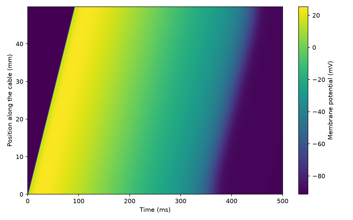
The membrane potential along the cable over time — Fig. 1 The membrane potential along the 50 mm cable over the first 500 ms, computed on a Tesla V100. The wave of excitation starts at the stimulated end at 0 mm and reaches the far end after about 90 ms. The cells repolarize about 360 ms after they were excited, so the wave of repolarization travels along the cable in the same way.#

The wave travels along the cable at about 0.55 m/s, which is within the range of the conduction velocity in human ventricles.

Troubleshooting#

main.cu checks every CUDA call and stops with the error CUDA reports. The common ones are:

`CUDA driver version is insufficient for CUDA runtime version`#

The program cannot use the GPU’s driver. Run nvidia-smi:

If it says No devices were found, or there is no nvidia-smi, no GPU is visible to the program. On a cluster you are probably on a login node, or in a job without a GPU: run on a GPU node, e.g. with srun --gres=gpu:1 ./cable v.csv (depending on the cluster). A Docker container needs --gpus all.
Otherwise, compare the CUDA Version in the top right of its output (the newest CUDA the driver supports) with nvcc --version. If nvcc is newer, e.g. CUDA 13.0 with a driver for CUDA 12.2, compile with an older CUDA (on a cluster often module avail cuda) or update the driver. Compiling with CUDA 12.x for a driver for an older CUDA 12 usually works, but CUDA 13 needs a driver for CUDA 13.

`no kernel image is available for execution on the device`#

The program was compiled for another GPU architecture than the one it runs on. Compile with -arch=native on the machine with the GPU, or with the architecture nvidia-smi reports (see above).

Note

CUDA 13 no longer supports Volta GPUs (V100) and older. For those, compile with CUDA 12 and -arch=sm_70.

Source code#
main.cu#// Solve a 1D cable of ToR-ORd cells on an NVIDIA GPU, with the kernels generated by
//
//   gotranx ode2cuda ToRORd_dyn_chloride.ode --scheme generalized_rush_larsen --namespace tor_ord -o tor_ord.cuh
//
// One GPU thread per cell. Each time step first advances every cell's ODE with the generated
// scheme, then lets the potential diffuse to the neighbouring cells (cable.cuh). Every
// millisecond the potential of every cell is written as one row of a CSV file.
//
// Build and run: nvcc -std=c++17 -O3 -arch=native -diag-suppress 177 main.cu -o cable && ./cable v.csv
#include <cstdio>
#include <cstdlib>
#include <vector>

#include "cable.cuh"
#include "tor_ord.cuh"

static void check(cudaError_t error, const char *call, int line)
{
    if (error != cudaSuccess) {
        std::fprintf(stderr, "%s failed (line %d): %s\n", call, line, cudaGetErrorString(error));
        std::exit(1);
    }
}
#define CHECK(call) check((call), #call, __LINE__)

static int lookup(int index, const char *name)
{
    if (index < 0) {
        std::fprintf(stderr, "No variable named '%s' in the model\n", name);
        std::exit(1);
    }
    return index;
}

int main(int argc, char *argv[])
{
    const char *output = argc > 1 ? argv[1] : "v.csv";
    const std::int64_t n_cells = 500;  // a 50 mm cable
    const double t_end = 500.0;        // ms
    const int threads = 128;
    const int blocks = static_cast<int>((n_cells + threads - 1) / threads);

    // The parameters are shared by all cells. The model's own stimulus would stimulate every
    // cell at once, so switch it off: the cable is stimulated at one end instead (cable.cuh)
    std::vector<double> parameters(tor_ord::NUM_PARAMS);
    tor_ord::init_parameter_values(parameters.data());
    parameters[lookup(tor_ord::parameter_index("i_Stim_Amplitude"), "i_Stim_Amplitude")] = 0.0;
    const int v = lookup(tor_ord::state_index("v"), "v");

    // The states of all cells, state-major: state i of cell c is states[i * n_cells + c], so
    // the potential of all cells is the contiguous row states + v * n_cells
    double *states, *d_parameters, *v_new;
    CHECK(cudaMalloc(&states, sizeof(double) * tor_ord::NUM_STATES * n_cells));
    CHECK(cudaMalloc(&d_parameters, sizeof(double) * tor_ord::NUM_PARAMS));
    CHECK(cudaMalloc(&v_new, sizeof(double) * n_cells));
    CHECK(cudaMemcpy(d_parameters, parameters.data(), sizeof(double) * tor_ord::NUM_PARAMS,
                     cudaMemcpyHostToDevice));
    tor_ord::init_state_values<<<blocks, threads>>>(states, n_cells);
    CHECK(cudaGetLastError());

    std::FILE *out = std::fopen(output, "w");
    if (out == nullptr) {
        std::fprintf(stderr, "Could not open %s\n", output);
        return 1;
    }
    std::vector<double> v_host(n_cells);
    double *potential = states + v * n_cells;

    const int num_steps = static_cast<int>(t_end / cable::dt);
    const int save_every = static_cast<int>(1.0 / cable::dt);  // every ms
    for (int step = 0; step <= num_steps; step++) {
        const double t = step * cable::dt;
        if (step % save_every == 0) {
            CHECK(cudaMemcpy(v_host.data(), potential, sizeof(double) * n_cells,
                             cudaMemcpyDeviceToHost));
            std::fprintf(out, "%g", t);
            for (std::int64_t c = 0; c < n_cells; c++) std::fprintf(out, ",%.6g", v_host[c]);
            std::fprintf(out, "\n");
        }
        // The cell model, in place: the scheme reads and writes the same states
        tor_ord::generalized_rush_larsen<<<blocks, threads>>>(states, t, cable::dt, d_parameters,
                                                             states, n_cells);
        CHECK(cudaGetLastError());
        // The diffusion of the potential, and the stimulus at the start of the cable
        cable::diffuse<<<blocks, threads>>>(potential, v_new, n_cells, cable::stimulus(t));
        CHECK(cudaGetLastError());
        CHECK(cudaMemcpy(potential, v_new, sizeof(double) * n_cells, cudaMemcpyDeviceToDevice));
    }
    CHECK(cudaDeviceSynchronize());

    std::fclose(out);
    CHECK(cudaFree(states));
    CHECK(cudaFree(d_parameters));
    CHECK(cudaFree(v_new));
    return 0;
}

cable.cuh#// A 1D cable of cardiac cells: the diffusion of the membrane potential between neighbouring
// cells, and the stimulus that starts a wave at one end. Used by main.cu, together with the
// cell model generated by `gotranx ode2cuda` (tor_ord.cuh).
#pragma once
#include <cstdint>

namespace cable
{
constexpr double dt = 0.01;  // ms, time step of both the cell model and the diffusion
constexpr double dx = 0.1;   // mm, distance between neighbouring cells
constexpr double D = 0.1;    // mm^2/ms, diffusion coefficient of the potential
constexpr double alpha = D * dt / (dx * dx);  // must be below 0.5 for stability

// The first cells are stimulated for the first millisecond, at the rate the model's own
// stimulus would raise the potential (its amplitude is -53 uA/uF, i.e. +53 mV/ms)
constexpr int n_stimulated = 5;
constexpr double stimulus_duration = 1.0;  // ms
constexpr double stimulus_rate = 53.0;     // mV/ms

// The increase of the potential of the stimulated cells in the step that starts at t
inline double stimulus(double t)
{
    return t < stimulus_duration ? stimulus_rate * dt : 0.0;
}

// One explicit step of dv/dt = D d^2v/dx^2 with no flux through the ends, from v into
// v_new, plus `stimulus` on the first n_stimulated cells. One thread per cell; v is the row
// of the potential in the state-major states, &states[v_index * n_cells].
static __global__ void diffuse(const double *v, double *v_new, const std::int64_t n_cells,
                        const double stimulus)
{
    const std::int64_t cell = static_cast<std::int64_t>(blockIdx.x) * blockDim.x + threadIdx.x;
    if (cell >= n_cells) return;

    // At the ends, the missing neighbour mirrors the existing one (no flux). A cable of one
    // cell has neither, and the cell is its own neighbour
    const bool has_left = cell > 0, has_right = cell < n_cells - 1;
    const double left = has_left ? v[cell - 1] : has_right ? v[cell + 1] : v[cell];
    const double right = has_right ? v[cell + 1] : has_left ? v[cell - 1] : v[cell];
    v_new[cell] = v[cell] + alpha * (left - 2.0 * v[cell] + right);
    if (cell < n_stimulated) v_new[cell] += stimulus;
}
}  // namespace cable

plot.py#"""Plot the potential along the cable over time, as written by main.cu (v.csv), into an
image next to it (v.png)."""

import sys
from pathlib import Path

import matplotlib.pyplot as plt
import numpy as np

dx = 0.1  # mm, as in cable.cuh

csv = Path(sys.argv[1] if len(sys.argv) > 1 else "v.csv")
data = np.loadtxt(csv, delimiter=",")
t, v = data[:, 0], data[:, 1:]
x = np.arange(v.shape[1]) * dx

fig, ax = plt.subplots(figsize=(8, 5))
image = ax.imshow(
    v.T,
    aspect="auto",
    origin="lower",
    extent=(t[0], t[-1], x[0], x[-1]),
    cmap="viridis",
)
ax.set_xlabel("Time (ms)")
ax.set_ylabel("Position along the cable (mm)")
fig.colorbar(image, ax=ax, label="Membrane potential (mV)")
fig.tight_layout()
fig.savefig(csv.with_suffix(".png"), dpi=150)

Solving a cable of cells on the GPU

Contents

Solving a cable of cells on the GPU#

Generating the CUDA code#

The cable#

Running the demo#

Troubleshooting#

`CUDA driver version is insufficient for CUDA runtime version`#

`no kernel image is available for execution on the device`#

Source code#

`main.cu`#

`cable.cuh`#

`plot.py`#

Solving a cable of cells on the GPU

Contents

Solving a cable of cells on the GPU#

Generating the CUDA code#

The cable#

Running the demo#

Troubleshooting#

CUDA driver version is insufficient for CUDA runtime version#

no kernel image is available for execution on the device#

Source code#

main.cu#

cable.cuh#

plot.py#

`CUDA driver version is insufficient for CUDA runtime version`#

`no kernel image is available for execution on the device`#

`main.cu`#

`cable.cuh`#

`plot.py`#