Comparing Linked Lists and Dynamic Arrays

Comparing Linked Lists and Dynamic Arrays#

In this chapter, we will apply the brief discussion about algorithm analysis and big O notation to two different cases. First, we will look at the differences between the linked list data structure and the dynamic array data structure. Then, we will further introduce different sorting algorithms, showing how they compare in terms of computational complexity.

Big O#

Recall from Algorithm Analysis and Big O notation that we introduced the big O notation to classify how much work an algorithm has to carry out to solve some problem, given the size of that problem. For sorting a list, for example, the size of the list would be the problem size. We often denote the problem size by $n$.

The main point we are interested in is understanding how the algorithm scales with the problem size as the problem grows. Does the computational cost grow linearly? Quadratically? Exponentially? This is where the big O notation comes in.

We find the big O complexity of an algorithm by finding the number of operations it has to carry out to solve some problem. However, instead of finding this exact number, we care only about the fastest-growing term while also disregarding any coefficients.

Using big O notation, we will classify most algorithms into one of the categories in the list below, which is organized from slowest-growing to fastest-growing. An algorithm that is $\mathcal{O}(1)$ scales perfectly: we can increase the problem size, and the time to solve it will not change! An algorithm that is $\mathcal{O(n)}$ scales linearly: if we double the problem size, we will roughly double the computation time. An algorithm that is $\mathcal{O}(e^n)$ scales horribly: as the problem size grows, the computation time grows exponentially. For larger inputs, this algorithm will stop working as we run out of computational resources.

Big O	Name
$\mathcal{O}(1)$	constant
$\mathcal{O}(\log n)$	logarithmic
$\mathcal{O}(n)$	linear
$\mathcal{O}(n \log n)$	loglinear/quasilinear
$\mathcal{O}(n^2)$	Quadratic
$\mathcal{O}(n^3)$	Cubic
$\mathcal{O}(n^k)$	Polynomial
$\mathcal{O}(e^n)$	Exponential
$\mathcal{O}(n!)$	Factorial

Computing with Big O#

Most algorithms consist of many different steps, which can be analyzed independently. The total cost of the algorithm is then the sum of the costs of each step. After finding the big O costs of each step, we then need to add the obtained expressions, as the next example illustrates

\[\mathcal{O}(n) + \mathcal{O}(n^2).\]

When adding big O expressions together, we simply keep the biggest term

\[\mathcal{O}(n) + \mathcal{O}(n^2) = \mathcal{O}(n^2).\]

Notice that having multiple elements with the same “biggest term” does not affect the final complexity, as adding these expressions together would just give a different coefficient, which is disregarded as in the example below

\[\mathcal{O}(1) + \mathcal{n} + \mathcal{n} = \mathcal{O}(n).\]

Similarly, sometimes we need to carry out an operation many times (when iterating or looping, for example). Consequently, we multiply the cost of each operation by the number of repetitions, such as

\[10\mathcal{O}(n^2).\]

This accounts, again, for a constant coefficient that gets ignored, meaning

\[10\mathcal{O}(n^2) = \mathcal{O}(n^2).\]

The exception to this procedure is if the number of steps is a function of the problem size $n$. For example, when iterating a list of size $n$ or performing $n$ multiplications. In that case, we need to multiply the number of repetitions by the big O complexity. Performing $n$ steps that each cost $\mathcal{O}(n)$, for example, results in a cost of

\[n \cdot \mathcal{O}(n) = \mathcal{O}(n^2).\]

Similarly, performing $n$ steps of an algorithm costing $\mathcal{O}(n\log n)$ gives a total cost of

\[n\cdot \mathcal{O}(n\log n) = \mathcal{O}(n^2 \log n).\]

The List ADT#

Previously, we created two different list classes: ArrayList and LinkedList. These two classes both implement the list abstract data type (ADT) but with two different data structures as their basis

The ArrayList is built on top of the dynamic array structure
The LinkedList is built on top of the linked list structure.

We will now look closer at how the different choice for the base data structure affects their performance. To do so, we will go through the different operations of the list ADT, such as insertions, removal, and indexing, all supported by both classes,

We will characterize the costs in terms of the length of the list, denoted $n$.

Appending#

Let us start with the operation of appending new elements to the end of the list. Both classes support this method, but what is the cost of appending?

Dynamic Array#

For a dynamic array, appending an element is the same as assigning that value to the first unused element of the underlying storage array. The cost of this operation is not dependent on the length of the list. It does not matter if the list has 100 or 100 million elements; appending a value is simply assigning a value to the next unused space. Thus, the cost of appending an element to our ArrayList is $\mathcal{O}(1)$.

However, sometimes there will not be any free space left in the underlying storage array. To resolve this corner case, we had to implement a “resize” operation which doubled the size of the underlying array. If the list has $n$ elements, this means we allocate an array of $2n$ elements in case the storage array is full. Then we copy over the $n$ elements of the array and deallocate the previous storage array. The bigger the list is, the more work this resizing takes. Specifically, the resize operation scales as $\mathcal{O}(n)$.

Having that said, appending to ArrayList only sometimes incurs the cost of a resize operation, so it is natural to question how to include this occasional cost in the analysis. While this question is left unanswered for now, we will simply say that the ArrayList.append method has a cost of $\mathcal{O}(1)$ with an occasional $\mathcal{O}(n)$.

Linked List#

Recall that appending an element to the linked list required starting at its “head” and iterating through to its end. The method looked something similar to

void append(int val)
{
    if (head == nullptr)
    {
        head = new Node(val);
        return;
    }

    Node *current = head;
    while (current->next != nullptr)
    {
        current = current->next;
    }
    current->next = new Node(val);
}

Since we iterate from the head of the list all the way to the end, we perform $n$ operations. If the list consists of 100 nodes, the loop needs to run 100 times, and once we get to the end, attaching the new node takes only a few operations. Thence, most of the work of appending to the LinkedList comes from iterating through the whole list, and the whole append method costs $\mathcal{O}(n)$.

Notice that because we need to iterate from the start of the list, the cost of appending more elements also grows as the list grows. If the size of the array doubles, then the cost of iterating through the array will double.

Comparing the two data structures#

We have seen that the appending method costs $\mathcal{O}(1)$ for the DynamicArray and $\mathcal{O}(n)$ for the LinkedList. This means that while the two might be equally fast for appending a few elements, as the lists grow, appending more elements to the linked list will become ever slower, while for the DynamicArray, it will stay the same.

This comparison might be seen as unfair, as the dynamic array also needed to occasionally resize, which is a costly operation. This indeed requires a closer analysis. Instead of referring to a single append operation, which will likely not incur a resize, let us look at a whole set of appends that definitely incur a resize. We can then find the “average cost” of an append, a concept called the amortized cost of an operation.

Amortized Cost#

The amortized cost of an operation is the average cost of a single operation when performed multiple times. This cryptic term comes from the world of finance and economics, taking inspiration from the fact that a business might amortize its costs by spreading them evenly throughout the year, for example. It is simply a way of averaging costs and payments.

Instead of analyzing a single append. Let us say we start with an empty dynamic array and append $n$ elements to it

ArrayList example;

for (int i = 0; i < n; i++)
{
    example.append(i);
}

What is the total cost of this operation, in big O, as a function $n$? Each of the $n$ appends cost $\mathcal{O}(1)$, so $n$ operations of $\mathcal{O}(1)$ will cost a total of $\mathcal{O}(n)$.

But what is the total cost of all the resizes required to reach $n$? This is better understood by starting from the end of the process and working backward to the start. The last required resize had to increase the underlying storage from $n/2$ to $n$, which costs $n$. The resize before that would need to take it from $n/4$ to $n/2$, costing $n/2$. The one before that would need to take it from $n/8$ to $n/4$, analogously with a cost of $n/4$, and so on. The total cost of all the resizes would therefore be

\[n + \frac{n}{2} + \frac{n}{4} + \frac{n}{8} + \ldots,\]

all the way down to the empty list. The exact number of resize operations will depend on what $n$ is.

This sum is a geometric progression, which sums out to $2n$. The easiest way to see this is to draw out the series as several boxes

In conclusion, while each resize might be costly, we carry out so few of them that the total cost of all the resizes also becomes $\mathcal{O(n)}$ and the total cost of appending $n$ elements to an empty DynamicArray is

\[\mbox{(cost of $n$ appends)} = \mathcal{O}(n) + \mathcal{O}(n) = \mathcal{O}(n).\]

If doing $n$ appends has a total cost of $\mathcal{O}(n)$, the average/amortized cost of a single operation must be

\[\mbox{(amortized cost of 1 append)} = \frac{1}{n}\cdot \mbox{(cost of $n$ appends)} = \frac{1}{n}\cdot \mathcal{O}(n) = \mathcal{O}(1).\]

Finally, on average, the cost of appending an element to our ArrayList is still not dependent on the size of that list, unlike for the linked lists.

Inserting elements into the front#

We have studied the cost of appending elements to the back of the list, but what about pushing them to the front? For our LinkedList, this was implemented as a push_front method or alternatively as the insert method specifying the index 0. While we did not implement this method for the ArrayList, it is part of project 2, so we will analyze its cost.

Dynamic Array#

To insert an element at the front of a dynamic array, we need to first make space for it by moving every other element in the list one index up. This operation requires moving the existing $n$ elements, costing $\mathcal{O}(n)$. After this is done, adding the new element is simple, only requiring a single assignment, incurring a cost of $\mathcal{O}(1)$. In total, appending to the front of a dynamic array is

\[\mathcal{O}(n) + \mathcal{O}(1) = \mathcal{O}(n).\]

Linked List#

For the linked list, we did implement the push_front method in an almost trivial manner because of the head pointer of the class pointing at the first element

void push_front(val)
{
    head = new Node(val, head);
}

This method is equally simple for 0, 10, or one million elements in the list. No matter the size of the list, it takes only a few operations, resulting in a cost of $\mathcal{O}(1)$.

Comparing the two data structures#

First, we saw that the cost of appending is constant ($\mathcal{O}(1)$) for a dynamic array but scales linearly ($\mathcal{O}(n)$) with the linked list. Now, we have seen that the reverse is true for adding elements to the front: the cost is constant for the linked list and linear for the array list!

Adding a Tail Pointer to the Linked List#

In the analysis of the linked list data structures so far, we have seen that adding an element to the front of the linked list is easier than adding it to the back. Indeed, the former had a cost of $\mathcal{O}(1)$ while the latter had a cost $\mathcal{O}(n)$. This is because, while we have the head pointer to the list’s first element, getting to its back requires us to iterate through the whole chain.

However, there is no reason we cannot also add a pointer to the end of the chain, using it as a shortcut to get there. This pointer is often called the tail pointer because it points to the tail of the list. If we have a tail pointer in our class, we can rewrite the append method as

void append(int val)
{
    if (head == nullptr)
    {
        head = new Node(val);
        tail = head;
    }
    else
    {
        tail->next = new Node(val);
        tail = tail->next;
    }
}

Implementing a tail point to the append method then makes it practically just as easy as the push_front method. Furthermore, by doing so, we improved the scaling of the append method to $\mathcal{O}(1)$, the same as for the DynamicArray.

Inserting into the middle#

So far, we have covered inserting into the back or to the front of the list. Nonetheless, we can also insert elements at some position in the middle of a list. Here, we do not necessarily mean the exact middle but a given index $i$.

Dynamic Array#

Inserting an element somewhere in the middle of the list is slightly easier than adding it to the front, as we only have to move the elements with indices larger than the index of insertion to make room. However, this still means moving something approximately half the elements of the list, i.e., $n/2$ elements, so the cost would still increase linearly with $n$ and still be $\mathcal{O}(n)$.

If we instead want to measure the cost as a function of both $n$ and $i$, then it would be

\[\mathcal{O}(n-i),\]

which shows that the further back in the list we want to insert, the bigger the index $i$, and the less the operation costs.

Linked List#

For a linked list, the insertion of a new node itself is not very costly; we only need to create a new node and hook it into the chain. The insertion itself would only cost $\mathcal{O}(1)$. However, just like appending (before adding the tail pointer), we first need to get to the right nodes to carry out this operation. This last step costs $\mathcal{O}(n)$, as we need to start at the front of the list and iterate to wherever the node is to be connected.

One might think we can fix this situation by adding another reference pointer, as was done for the tail element. Unfortunately, this is not feasible for a general index $i$ as it would require us to make another list to store all those reference pointers.

However, as the cost of inserting is itself $\mathcal{O}(1)$, we might be able to piggyback off other algorithms and methods that iterate through the list anyway. For a dynamic array, this is not possible because regardless of how the element is obtained, the cost comes from having to move all the other elements to make room.

Summarizing#

Operation	Dynamic Array	Linked List	Linked list (w/ tail ref)
Insert at back	$\mathcal{O}(1)^*$	$\mathcal{O}(n)$	$\mathcal{O}(1)$
Insert at front	$\mathcal{O}(n)$	$\mathcal{O}(1)$	$\mathcal{O}(1)$
Insert in middle	$\mathcal{O}(n)$	$\mathcal{O}(n)$	$\mathcal{O}(n)$

*) This is the amortized cost, i.e., the cost averaged over many operations

To summarize, the cost of inserting elements into the lists is different depending on what data structure we use. From the table above, it might seem that using a linked list with a tail pointer is the most efficient. This would indeed be the case if we were looking only at insertions; however, lists are not only used for insertions.

Indexing#

An important characteristic of using lists is that we can use indexing to read and write to list elements. We implemented this operation for both of our lists by overloading the square-bracket operator. Let us now study the cost of this operation.

Dynamic Array#

We implemented the indexing operator approximately like the following

int &operator[](int index)
{
    return data[index];
}

Because our data is actually stored in an underlying storage array (called data in this example), indexing our ArrayList is just an alias for indexing the underlying array.

One of the strengths of arrays is that the data lies contiguously in memory, and as we have seen earlier, indexing an array is just fancy memory address operations. If we write x[10] to get the 10’th element of some array, for example, then x is just a pointer/memory address with the indexing operations meaning *(x + 10). This represents some pointer arithmetic followed by the lookup of the value at the right memory address.

Arrays are contiguous in memory, so accessing any element by its index is trivial, as C++ computes its way to the correct memory address and looks up the right value. This is true regardless of the size of the array. Therefore, accessing an element by index in an array is $\mathcal{O(1)}$.

Because our ArrayList is built on top of arrays, our indexing operation will also be $\mathcal{O}(1)$.

Linked Lists#

For linked lists, the situation is different. The elements, i.e., nodes of a linked list, are not stored contiguously in memory. Each node can, for all intents and purposes, exist somewhere completely different in memory. What is paramount is that each node knows where the next one is stored.

This means that to get to an element based on its index $i$, we have to start at the front of the list and iterate all the way to the right element. We implemented this as something like

int &operator[](int index)
{
    Node *current = head;

    for (int i = 0; i < index; i++)
    {
        current = current->next;
    }
    return current;
}

In this code, we start at the head of the list and move $i$ steps, where $i$ is the index. This means accessing an element by index costs $\mathcal{O}(i)$. Often we do not express costs in terms of indices, so we simply say that this costs $\mathcal{O}(n)$. The larger the list, the bigger the index we typically access and the more costly it will be.

Indexing the final element in the list, for example, requires us to iterate through the entire list. If we have a tail reference, getting to the last element is easy, but getting to the second-to-last element is still hard. The difficulty comes from the fact that, while we have a tail reference, there is no way to iterate backward in the linked list. If we had implemented a doubly linked list, we could iterate from either side of the array. This would improve things somewhat, but for most indices, we would still need considerable iterations to get to a given index.

Comparing the two data structures#

For arrays and dynamic arrays, indexing is a “free” operation. It does not matter what index we want to access either. This is often referred to as random access. The name implies that it does not matter in what order we access the list elements; it might as well be random. A better name for it is direct access, implying we can directly access any element by its index. The reader might be familiar with the term random access memory (RAM), which refers to the normal memory on the computer, and has this name because accessing any part of it takes roughly the same amount of time.

As we have seen, a linked list is not a direct access data structure. We cannot access any given index directly but have to iterate through the sequence from the start. This is known as sequential access.

Summarizing#

Our findings are summarized in the table below. By analyzing the costs of the different operations, we can see how the data structures affect the overlying data type. While both data structures can support the same list ADT, the performance will differ.

Operation	Array	Dynamic Array	Linked List	Linked list (w/ tail ref)
Insert at back	-	$\mathcal{O}(1)^*$	$\mathcal{O}(n)$	$\mathcal{O}(1)$
Insert at front	-	$\mathcal{O}(n)$	$\mathcal{O}(1)$	$\mathcal{O}(1)$
Insert in middle	-	$\mathcal{O}(n)$	$\mathcal{O}(n)$	$\mathcal{O}(n)$
Get element by index	$\mathcal{O}(1)$	$\mathcal{O}(1)$	$\mathcal{O}(n)$	$\mathcal{O}(n)$

*) This is the amortized cost, i.e., the cost averaged over many operations

What we have not analyzed#

Our analysis has not been too extensive; we have simply compared some of the most important operations in terms of big O notation. Still, there are other important comparisons between the data structures, namely the difference in memory usage or other operations, such as removing elements. Another important difference is that, in practice, arrays are often fast because having contiguous elements in memory, allows them to be loaded into the CPU cache faster. Facts such as these are hard to include in our algorithm analysis.

While our analysis is simplified and theoretical, it is still very useful. Similar analyzes are often an essential part of algorithms and data structures.

Final recommendation#

For scientific computing, dynamic arrays usually win out in efficiency because of their contiguous memory storage. In practice, therefore, one might rarely need to use linked lists.

However, knowing how to implement and analyze linked lists is still a valuable skill, as they are an important introductory data structure and something one is expected to know about if ever moving further into computational science.

Some Analogies#

The major differences between linked lists and array lists revolve around how elements are added, removed, and read. This can be a very abstract concept, so many people like to make analogies to understand and remember the differences.

For instance, when it comes to indexing, an example of a linked list would be the alphabet. Few people can directly answer the question “Which letter is the 17th in the alphabet?” because most people cannot “index” the alphabet. Instead, they have to start at the beginning and count their way to the 17th letter/element. However, the question “Which letter comes after P in the alphabet?” can be easily answered.

Similarly, indexing an array can be thought of as indexing the pages in a book. When asked to open a book to page number 277, one would not have to start on page 1 and flip each page to get to the right spot. Instead, one could go directly to the right page.

We can also talk about adding/removing elements. An analogy for adding elements to a dynamic array could be adding a book to a stack of books lying on a table. Adding a book to the end of the stack is easy: just place it on top where there is room. However, inserting the book into the bottom or middle of the pile requires a lot more work. The bigger the stack, the more work.

../../../_images/stack_of_books.jpg — Fig. 38 A dynamic array is like a stack of books.#

Adding or removing elements from a linked list can be thought of as modifying a chain, such as a bicycle chain. To lengthen a bike chain, one simply disconnects two of the “nodes” of the chain, adds in some more, and puts them back together. It does not matter how long the chain is; adding more chains is equally hard. For the insert “into the middle” method, we also added the “search time” to get to the right node. This would be analogous to a bike chain with a broken node. First, one would need to find the broken linker by “iterating” through the chain, then one removes the broken linker and puts a new one in.

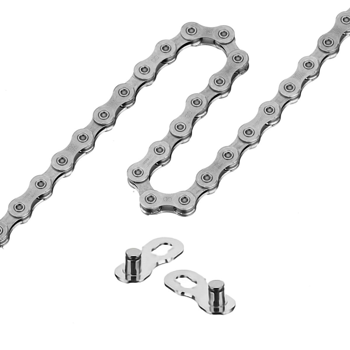
../../../_images/bike_chain.jpg — Fig. 39 A linked list is like a bike chain.#

Operation	Dynamic Array	Linked List	Linked list (w/ tail ref)
Insert at back	\(\mathcal{O}(1)^*\)	\(\mathcal{O}(n)\)	\(\mathcal{O}(1)\)
Insert at front	\(\mathcal{O}(n)\)	\(\mathcal{O}(1)\)	\(\mathcal{O}(1)\)
Insert in middle	\(\mathcal{O}(n)\)	\(\mathcal{O}(n)\)	\(\mathcal{O}(n)\)

Operation	Array	Dynamic Array	Linked List	Linked list (w/ tail ref)
Insert at back	-	\(\mathcal{O}(1)^*\)	\(\mathcal{O}(n)\)	\(\mathcal{O}(1)\)
Insert at front	-	\(\mathcal{O}(n)\)	\(\mathcal{O}(1)\)	\(\mathcal{O}(1)\)
Insert in middle	-	\(\mathcal{O}(n)\)	\(\mathcal{O}(n)\)	\(\mathcal{O}(n)\)
Get element by index	\(\mathcal{O}(1)\)	\(\mathcal{O}(1)\)	\(\mathcal{O}(n)\)	\(\mathcal{O}(n)\)

Big O	Name
\(\mathcal{O}(1)\)	constant
\(\mathcal{O}(\log n)\)	logarithmic
\(\mathcal{O}(n)\)	linear
\(\mathcal{O}(n \log n)\)	loglinear/quasilinear
\(\mathcal{O}(n^2)\)	Quadratic
\(\mathcal{O}(n^3)\)	Cubic
\(\mathcal{O}(n^k)\)	Polynomial
\(\mathcal{O}(e^n)\)	Exponential
\(\mathcal{O}(n!)\)	Factorial

Comparing Linked Lists and Dynamic Arrays

Contents

Comparing Linked Lists and Dynamic Arrays#

Big O#

Computing with Big O#

The List ADT#

Appending#

Dynamic Array#

Linked List#

Comparing the two data structures#

Amortized Cost#

Inserting elements into the front#

Dynamic Array#

Linked List#

Comparing the two data structures#

Adding a Tail Pointer to the Linked List#

Inserting into the middle#

Dynamic Array#

Linked List#

Summarizing#

Indexing#

Dynamic Array#

Linked Lists#

Comparing the two data structures#

Summarizing#

What we have not analyzed#

Final recommendation#

Some Analogies#