Solving the 1D Diffusion Equation using Finite Differences#
In Random Walks we looked at random walks and finished the discussion by showing how to go from a discrete problem to a continuous partial differential equation called the Diffusion Equation.
The following text briefly presents a specific method for solving this equation numerically and looks at some solutions with different initial conditions and boundary conditions. Most of the material here is presented as supplementary and is not considered part of IN1910’s curriculum.
Solving the Diffusion Equation using Finite Differences#
A popular strategy for solving both ODEs and PDEs is discretizing them so that we only solve them at regular intervals, called mesh points. The derivatives are then approximated with ‘finite’ differences, as opposed to the infinitesimal limit they actually represent.
This process is called discretizing the continuous differential equations and is the exact opposite process of what we did to find the PDE in the first place!
We denote the desired solution by \(c(x,t)\) because it can be interpreted as the concentration of some particles at a given location \(x\) at time \(t\). An example could be the concentration of oxygen in a room.
The function is discretized using a given step length \(\Delta x\) in space and a given time step \(\Delta t\) in time. Thus, we will only solve for the concentration at points
where \(i\) and \(j\) are integers. To simplify writing, we define the shorthand
Approximating the derivative of the above equation can be done in many ways. The most straightforward method is to use only the first terms of the Taylor series, which leads to the expression found in Random Walks,
Note, however, that this yields a first-order finite difference approximation in time but a second-order finite difference order in space. Consequently, the intervals should be such that \(\Delta t \leq \Delta x.\)
Approximating the spatial derivative#
For the spatial derivative, we use a second-order central difference approximation
This is again found from truncating the Taylor series, but this time the error is \(\mathcal{O}(\Delta x^2)\), meaning the solver will be more accurate to the second-order spatial step length compared to the first-order time step. This means we should pick \(\Delta t < \Delta x\).
Finding our computational stencil#
The numerical expression is now
This expression can be simplified even further. By shuffling around some terms, we get
Remember that \(D\), \(\Delta t\), and \(\Delta x\) are all constants, so we can also introduce a new constant
which results in the equation
or
Such an equation is sometimes shown as a computational stencil
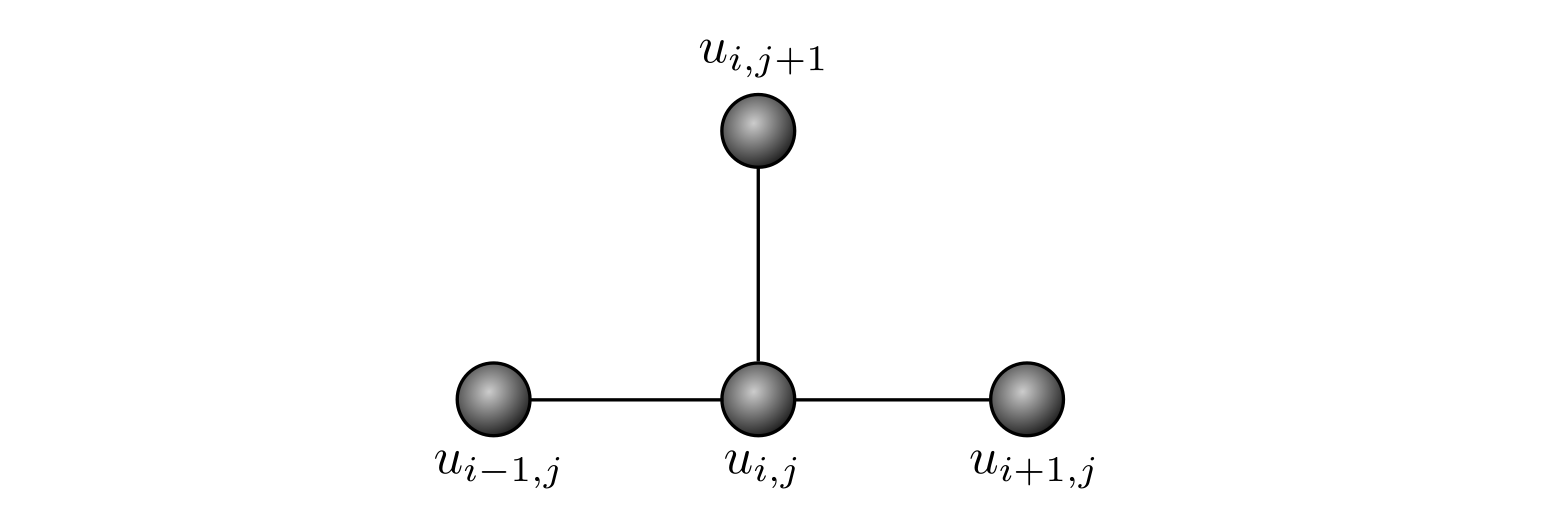
Looking at the equation or the stencil, it is clear that we compute the concentration at the ‘next’ time step \(t_{j+1}\), based on the values at the ‘current’ time step \(t_j\), with respect to the three closest points in space \(x_{i-1}\), \(x_i\) and \(x_{i+1}\).
Explicit vs. Implicit#
Note that the computational stencil only involves a single ‘next’ time step. This is called an explicit scheme, as it explicitly states how to compute the new values. The opposite would be an implicit scheme, where for each time step, the solver must algebraically solve a set of equations to find the new values. Simply put, explicit schemes are significantly easier to implement and solve. The downside is that explicit schemes can sometimes be unstable, requiring more carefulness with the computational resolution. Some implicit schemes, such as the backward Euler scheme, are much more stable and can handle a wider variety of parameters and resolutions.
Handling the boundaries#
Looking at the stencil, it is clear there will be an issue at the boundaries of the domain. To calculate the point at the edge of the boundary, \(u_{0, j+1}\), we need to know \(u_{-1, j+1}\), which does not exist! To get around this problem, boundary conditions need to be specified.
The simplest boundary conditions are the Dirichlet conditions, also known as a concentration clamp. This simply forces the solution to have certain values at the boundary, named clamped values: \(u(0, t) = u_0\) and \(u(L, t) = u_L\). Consequently, those values do not need to be computed.
The other common set of boundary conditions is the Neumann conditions. With these, the flux over the boundary is clamped and not the concentration itself. Most commonly, the flux is set to 0, meaning no concentration can ever cross the boundary. This specific condition is often referred to as a ‘no-flow’ or ‘reflective’ boundary. To implement this condition, we introduce points immediately outside the boundary, \(u_{-1, j}\), and set these imaginary ‘ghost points’ to have the same value as the actual boundary. As a diffusion flux is driven by a concentration difference, by setting \(u_{-1,j} = u_{0,j}\), the math itself will make sure no flux occurs across the boundary.
Implementing the Solver#
Now that the mathematical basis has been discussed, it is possible to implement the solver. We start by importing the required packages.
import numpy as np
import matplotlib.pyplot as plt
from matplotlib import animation, rc
from IPython.display import HTML

%matplotlib inline
A note on stability#
Here we have chosen to use a forward Euler scheme because it is easy to describe briefly. It is also straightforward to implement, thanks to it being an explicit scheme. However, it has a significant error compared to other methods and, more importantly, is unstable. Being unstable means it will produce a completely wrong answer to the equation for certain parameters. Mathematical analysis shows that the stability criterion for this scheme is
To ensure stability, the following simulations use \(D=5\), \(\Delta x = 0.5\) and \(\Delta t = 0.02\), giving \(\alpha = 0.4\).
D = 5
dx = 0.5
dt = 0.020
alpha = D * dt / dx / dx

# Double check stability
if alpha > 0.5:
    raise ValueError("The scheme is not stable with the chosen parameters.")
else:
    print(alpha)
0.4
We now implement a function we can call to update the solution by one time step. The differential equation should not be solved for the boundaries, as their value is system-specific. Therefore, the implemented function will only update the internal points.
def step(u):
    """A function that iterates the solution one step in time.
    Note: This function does not enforce any boundary conditions."""
    up[:] = u[:]
    u[1:-1] = alpha * up[2:] + (1 - 2 * alpha) * up[1:-1] + alpha * up[:-2]
With the step function defined, we are ready to solve specific systems.
System 1: An initial concentration spike#
The first system to be considered is one where there is an initial spike of concentration in the middle of a domain. First, we explore the situation where the domain has open boundaries so that the concentration can escape from the box. Subsequently, we change to reflective boundaries so that nothing can escape from the box.
# Define the spatial mesh
L = 10
x = np.arange(0, L + dx, dx)
n = len(x)

# Set up arrays to hold the solution at the current and previous time steps
u = np.empty(n)
up = np.empty(n)
Open Boundaries#
As mentioned, assuming the domain has open boundaries, the concentration can escape from the box.
%%capture

# Set up initial condition
u[:] = 0
u[n // 2 - 1 : n // 2 + 1] = 4

fig, ax = plt.subplots()
ax.set_xlim((0, L))
ax.set_ylim((0, 2))
(line,) = ax.plot(x, u, linewidth=2)


def animate(i):
    # Calculate solution for next time step
    step(u)
    u[0] = 0
    u[-1] = 0

    # Update plot
    line.set_ydata(u)
    return (line,)


anim = animation.FuncAnimation(fig, animate, repeat=False, frames=400, interval=20)
HTML(anim.to_html5_video())
---------------------------------------------------------------------------
RuntimeError                              Traceback (most recent call last)
Cell In[6], line 1
----> 1 HTML(anim.to_html5_video())

File /opt/hostedtoolcache/Python/3.10.12/x64/lib/python3.10/site-packages/matplotlib/animation.py:1284, in Animation.to_html5_video(self, embed_limit)
   1281 path = Path(tmpdir, "temp.m4v")
   1282 # We create a writer manually so that we can get the
   1283 # appropriate size for the tag
-> 1284 Writer = writers[mpl.rcParams['animation.writer']]
   1285 writer = Writer(codec='h264',
   1286                 bitrate=mpl.rcParams['animation.bitrate'],
   1287                 fps=1000. / self._interval)
   1288 self.save(str(path), writer=writer)

File /opt/hostedtoolcache/Python/3.10.12/x64/lib/python3.10/site-packages/matplotlib/animation.py:148, in MovieWriterRegistry.__getitem__(self, name)
    146 if self.is_available(name):
    147     return self._registered[name]
--> 148 raise RuntimeError(f"Requested MovieWriter ({name}) not available")

RuntimeError: Requested MovieWriter (ffmpeg) not available
Reflective boundaries#
We now change to no-flow boundaries so that nothing can escape from the box.
%%capture

# Set up initial condition
u[:] = 0
u[n // 2 - 1 : n // 2 + 1] = 4

# Set up plot
fig, ax = plt.subplots()
ax.set_xlim((0, L))
ax.set_ylim((0, 2))
(line,) = ax.plot(x, u, linewidth=2)


def animate(i):
    # Calculate solution for next time step
    step(u)
    u[0] = (1 - alpha) * up[0] + alpha * up[1]
    u[-1] = (1 - alpha) * up[-1] + alpha * up[-2]

    # Update plot
    line.set_ydata(u)
    return (line,)


anim = animation.FuncAnimation(fig, animate, repeat=False, frames=400, interval=20)
HTML(anim.to_html5_video())
---------------------------------------------------------------------------
RuntimeError                              Traceback (most recent call last)
Cell In[8], line 1
----> 1 HTML(anim.to_html5_video())

File /opt/hostedtoolcache/Python/3.10.12/x64/lib/python3.10/site-packages/matplotlib/animation.py:1284, in Animation.to_html5_video(self, embed_limit)
   1281 path = Path(tmpdir, "temp.m4v")
   1282 # We create a writer manually so that we can get the
   1283 # appropriate size for the tag
-> 1284 Writer = writers[mpl.rcParams['animation.writer']]
   1285 writer = Writer(codec='h264',
   1286                 bitrate=mpl.rcParams['animation.bitrate'],
   1287                 fps=1000. / self._interval)
   1288 self.save(str(path), writer=writer)

File /opt/hostedtoolcache/Python/3.10.12/x64/lib/python3.10/site-packages/matplotlib/animation.py:148, in MovieWriterRegistry.__getitem__(self, name)
    146 if self.is_available(name):
    147     return self._registered[name]
--> 148 raise RuntimeError(f"Requested MovieWriter ({name}) not available")

RuntimeError: Requested MovieWriter (ffmpeg) not available
System 2 - Transport across the synaptic cleft#
For our second system, we will look at the diffusive transport of neurotransmitters across a synapse. When a signal is sent from one neuron to another, an action potential in the pre-synaptic membrane causes the release of neurotransmitter molecules into the synaptic cleft between the cells.
To model this system, we assume the concentration to be zero initially. At time \(t=0\), the pre-synaptic side, placed on the left, starts releasing neurotransmitters. For simplicity, this process is implemented as a concentration clamp \(u(0, t) = C\) on the left and \(u(L, t)=0\) on the right. The clamp in the pre-synaptic side implies the release of neurotransmitters is an equilibrium process, while the second clamp means the neurotransmitters are absorbed so rapidly that there are no unabsorbed neurotransmitters at this boundary. It is important to notice those are simplification assumptions to model the problem.
%%capture

# Pre-synaptic concentration
C = 5

# Set up initial condition
u[:] = 0

fig, ax = plt.subplots()
ax.set_xlim((0, L))
ax.set_ylim((0, C))
(line,) = ax.plot(x, u, linewidth=2)


def animate(i):
    # Calculate solution for next time step
    step(u)
    u[0] = C
    u[-1] = 0

    # Update plot
    line.set_ydata(u)
    return (line,)


anim = animation.FuncAnimation(fig, animate, repeat=False, frames=300, interval=20)
HTML(anim.to_html5_video())
---------------------------------------------------------------------------
RuntimeError                              Traceback (most recent call last)
Cell In[10], line 1
----> 1 HTML(anim.to_html5_video())

File /opt/hostedtoolcache/Python/3.10.12/x64/lib/python3.10/site-packages/matplotlib/animation.py:1284, in Animation.to_html5_video(self, embed_limit)
   1281 path = Path(tmpdir, "temp.m4v")
   1282 # We create a writer manually so that we can get the
   1283 # appropriate size for the tag
-> 1284 Writer = writers[mpl.rcParams['animation.writer']]
   1285 writer = Writer(codec='h264',
   1286                 bitrate=mpl.rcParams['animation.bitrate'],
   1287                 fps=1000. / self._interval)
   1288 self.save(str(path), writer=writer)

File /opt/hostedtoolcache/Python/3.10.12/x64/lib/python3.10/site-packages/matplotlib/animation.py:148, in MovieWriterRegistry.__getitem__(self, name)
    146 if self.is_available(name):
    147     return self._registered[name]
--> 148 raise RuntimeError(f"Requested MovieWriter ({name}) not available")

RuntimeError: Requested MovieWriter (ffmpeg) not available
Steady State Solution#
Eventually, the solution hits a pseudo-steady state, where the solution is no longer changing. This is because the solution has become a linear solution, \(c=Ax + b\) which means that
We call such a situation a pseudo-steady state because it looks like nothing is changing, but there is a constant flux of neurotransmitter molecules through the cleft.
We could have found this steady-state analytical solution for the diffusion equation using the fact that it is unchanging in time
giving
Adding in the boundary conditions of \(c(0) = C\) and \(c(L) = 0\) gives
Interestingly, the steady-state solution does not depend on the diffusion coefficient, \(D\), at all! However, the diffusion coefficient models how fast the system reaches the steady state and will enter into the net transport of neurotransmitters through Ficks law: \(J = -D \nabla c = CD/L\).
Shutting off the source#
Assume that the system has had enough time to reach steady-state condition. Eventually, the release event will stop, which is modeled by changing the concentration clamp on the left to a no-flow boundary instead. We assume the right-hand side keeps absorbing molecules.
%%capture

# Set up initial condition
u[:] = C * (1 - x / L)

fig, ax = plt.subplots()
ax.set_xlim((0, L))
ax.set_ylim((0, C))
(line,) = ax.plot(x, u, linewidth=2)


def animate(i):
    # Calculate solution for next time step
    step(u)
    u[0] = (1 - alpha) * up[0] + alpha * up[1]
    u[-1] = 0

    # Update plot
    line.set_ydata(u)
    return (line,)


anim = animation.FuncAnimation(fig, animate, repeat=False, frames=600, interval=20)
HTML(anim.to_html5_video())
---------------------------------------------------------------------------
RuntimeError                              Traceback (most recent call last)
Cell In[12], line 1
----> 1 HTML(anim.to_html5_video())

File /opt/hostedtoolcache/Python/3.10.12/x64/lib/python3.10/site-packages/matplotlib/animation.py:1284, in Animation.to_html5_video(self, embed_limit)
   1281 path = Path(tmpdir, "temp.m4v")
   1282 # We create a writer manually so that we can get the
   1283 # appropriate size for the tag
-> 1284 Writer = writers[mpl.rcParams['animation.writer']]
   1285 writer = Writer(codec='h264',
   1286                 bitrate=mpl.rcParams['animation.bitrate'],
   1287                 fps=1000. / self._interval)
   1288 self.save(str(path), writer=writer)

File /opt/hostedtoolcache/Python/3.10.12/x64/lib/python3.10/site-packages/matplotlib/animation.py:148, in MovieWriterRegistry.__getitem__(self, name)
    146 if self.is_available(name):
    147     return self._registered[name]
--> 148 raise RuntimeError(f"Requested MovieWriter ({name}) not available")

RuntimeError: Requested MovieWriter (ffmpeg) not available