Software Optimization

Software Optimization#

The word optimization gets thrown around, but let us try to narrow down what we mean by it.

Optimize — Make the best or most effective use of (a situation or resource).

Software optimization is clearly distinguished from mathematical optimization. Put simply, mathematical optimization is finding the maxima or minima of some mathematical function and its corresponding parameters. This kind of optimization is also an important topic and is often related to numerical methods such as Newton’s method. It is crucial to be clear about what kind of optimization we deal with.

This section will deal with software optimization. Our goal is to create more efficient programs. There are several different types of optimization in programming, but we will mainly focus on optimizing speed. Other possible optimization examples are memory, battery usage, and the number of code lines.

Example of software optimization: Google Video vs. YouTube#

During 2005-2006, there was a “feature war” between two online video-sharing platforms, Google Video and YouTube. Google Video was a large project with substantial investment: hundreds of developers and virtually unlimited hardware resources. On the other hand, YouTube was a small start-up with 20 developers. Each time YouTube implemented a new feature, it would take Google a month or two to implement something similar. Each time Google announced something new, it would take YouTube a week!

Why? In an interview, Alex Martelli, an engineer at Google, said, “The solution was very simple! Those 20 guys were using Python. We were using C++.”

One could say that Google Video was more optimized concerning performance, while YouTube was more optimized concerning implementation time.

Approximating \(\pi\)#

Let us start with a toy example, approximating \(\pi\). We introduce the Leibniz formula

\[ \frac{\pi}{4}= \sum\limits_{i=0}^{\infty} \frac{(-1)^{i}}{2i+1}, \]

which is derived from the Taylor series of \(\text{arctan}(x)\). To approximate \(\pi\), we can sum the \(N\) first terms of this series and multiply this by 4. We will compare Python and C++ algorithms with the same number of terms, \(N=123456789\).

Python#

def estimate_pi(N: int) -> float:
    pi_fourth = 0.0
    for i in range(N):
        pi_fourth += (-1.0) ** i / (2.0 * i + 1.0)
    return 4 * pi_fourth

import numpy as np

pi_estimated = estimate_pi(1000)
print("Estimated pi:", pi_estimated)
print("Error:", abs(np.pi - pi_estimated))

Estimated pi: 3.140592653839794
Error: 0.000999999749998981

It seems that the estimation works. With \(N=123456789\), this algorithm takes 14.49 seconds to run. Notice that this measured time is dependent on the local machine and might take a different time in case the reader tries to run it.

C++#

Can this be done even faster? Let us implement the same algorithm in C++.

#include <cmath>
#include <iomanip>
#include <iostream>
#include <string>

double estimate_pi(unsigned int N)
{
    double pi_fourth = 0.0;
    for (unsigned int i = 0; i < N; i++)
    {
        pi_fourth += std::pow(-1, i) * 1.0 / (2.0 * i + 1.0);
    }
    return 4.0 * pi_fourth
}

This C++ code does the same as the Python code and will output the same estimate to machine precision. For the same \(N=123456789\), the C++ code takes 0.60 seconds to run, whereas the compiling accounts for about 0.40 seconds, while the actual run time is approximately 0.20 seconds. This is a significant improvement on the Python code.

NumPy#

A third option is to use the Python package NumPy.

import numpy as np


def estimate_pi_numpy(N):
    sign = np.ones(N)
    sign[1::2] = -1
    i = np.arange(N)
    return 4 * np.sum(sign * (1 / (2 * i + 1)))

Using Python’s built-in slicing arr[start:stop:step], the line sign[1::2] = -1 sets the value -1 to every second element in sign, starting at index one. Then we define an indexing array, i, and finally, sum over all the elements using np.sum(). First, we show that this function outputs the same as the previous Python function.

pi_estimated = estimate_pi_numpy(1000)
print("Estimated pi:", pi_estimated)
print("Error:", abs(np.pi - pi_estimated))

Estimated pi: 3.140592653839792
Error: 0.0009999997500012014

So how does this runtime compare to the others when \(N=123456789\)? It only takes 0.83 seconds! That is almost as fast as the C++ code, but we still have the luxury of coding in Python. This is the case since NumPy is primarily coded in C or C++.

When to optimize?#

The first question we want to look at is when to optimize code. Ideally, we would write efficient and optimal code from the start. Most proficient programmers recommend optimizing after having developed code that works. Kent Beck, the creator of the software development methodology extreme programming, formulated this statement as

Make it Work
Make it Right
Make it Fast

Let us look at each step separately

1. Make it Work#

When solving a brand new problem or implementing a new feature, one cannot possibly focus on everything at once. A significant goal in programming is to work incrementally. Therefore, when solving a problem, we should ignore optimization and instead focus on the basics.

During problem-solving, we must verify that it works through verification and validation. This is done through rigorous testing. Writing an extensive test suite of test cases, unit tests, and integration tests can make us confident that we have a working solution.

2. Make it Right#

After breaking down the problem and creating a solution that seems to work, the next step is to make it “right” or “elegant”.

Making the code elegant refers to everything other than the code’s functionality. The central part of this step is referred to as refactoring code. Refactoring code means rewriting it, not to change its function, but to improve it in other ways.

Refactoring can include changing the overall structure of the code, for example, splitting code into functions, classes, or modules. It can also mean rewriting single lines or changing variable names. The goals are simple: making the code more structured and readable. The benefits are that the code is easier to read, understand, maintain, and develop.

By continuously improving the design of code, we make it easier and easier to work with. This is in sharp contrast to what typically happens: little refactoring and a great deal of attention paid to expediently adding new features. If you get into the hygienic habit of refactoring continuously, you’ll find that it is easier to extend and maintain code.

-Joshua Kerievsky, Refactoring to Patterns [].

When refactoring code, one should also look closely at the code style. It is common to ignore style guides during problem-solving. After the problem is solved, one should always review that the style is consistent and solid.

Another important part of making code elegant is to write good documentation, specifically docstrings in Python. Since the code may change during problem-solving, this step should wait until the code is developed and refactored. The main point is that wrong documentation is worse than no documentation.

After making the code more elegant through refactoring and rewriting, all tests from Make it Work should be rerun. This is because the rewriting might have broken the code. By rerunning the tests, we can verify that the program’s behavior is unchanged. This also emphasizes how important it is to implement good and extensive tests.

3. Make it Fast#

Now, we are finally at the optimization step. The important point is that it is placed after developing a working and elegant code.

We will turn to how to make the code faster shortly. However, it is also important to emphasize that if we make changes to our code to make it more effective and faster, we should rerun tests and verify that our changed solution still solves the problem and that we have not broken it in our strive for speed.

Should one Optimize?#

The third step above was formulated as “Make it Fast”. However, before making it fast, we should ask ourselves: Should we even optimize? Optimizing code is tricky, and while making the code faster, we are paradoxically spending time. If the goal of optimizing the code is to save time, one needs to save more time with the optimized code than the time it takes to perform the changes.

The XKCD comic below illustrates this point by showing how much time one can invest into optimizing the code and still save time. As the comic illustrates, how much time one saves by optimizing depends on how many times the code is run.

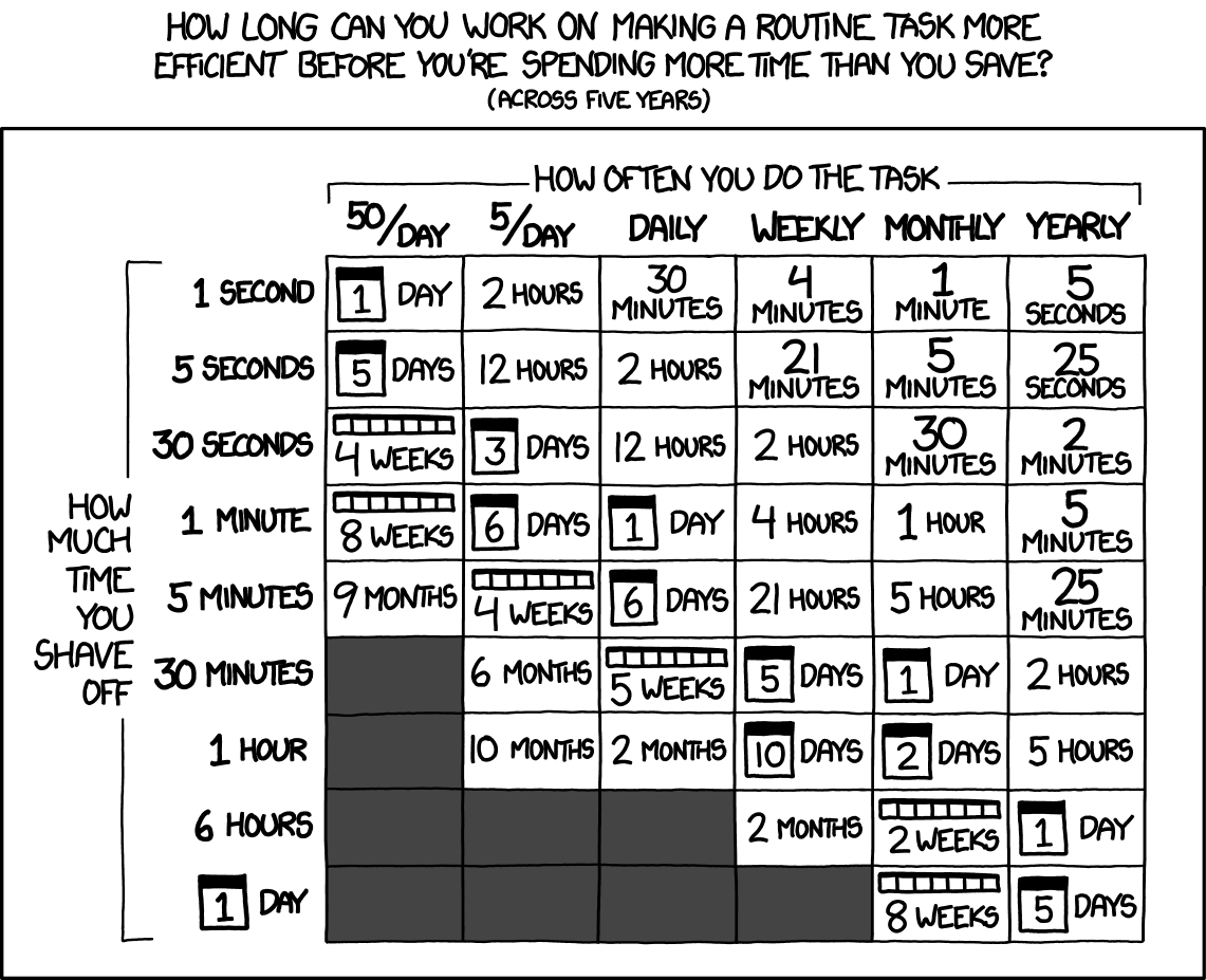
xkcd1205 — Fig. 58 **Source:** XKCD #1205#

It is important to stress that if the goal is to produce code to be shared with others or sold, making the code more efficient makes a better product. The goal is not to save the developers time but save others time. The table above is more from the point of view of writing and using code ourselves. In addition, sometimes optimization is done as a learning exercise, in which case the time used in the optimization is not “wasted time.” In other cases, it is about showing off or winning programming competitions.

xkcd974 — Fig. 59 **Source:** XKCD #974#

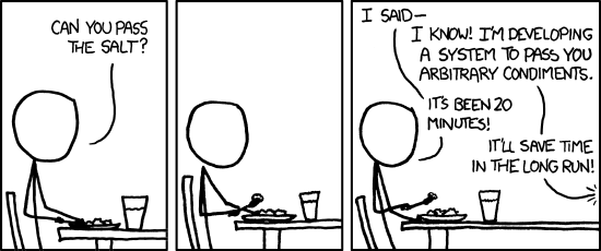
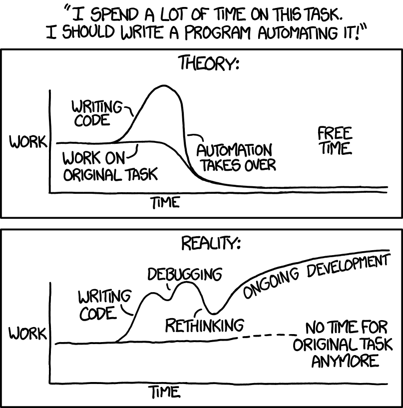
xkcd1319 — Fig. 60 **Source:** XKCD #1319#

Benefits of optimization#

Making programs run faster is not only about saving time. In scientific programming, faster code allows us to carry out experiments at a larger scale, with better precision, or run more experiments. Optimizing for speed is therefore important in that it not only enables us to do things faster, but it enables us to do more things.

Drawbacks of optimization#

While optimizing and making more efficient code sounds excellent, it is important to remember that it has drawbacks.

The first drawback is that it requires a lot of development time, as already mentioned. This development time could have instead been invested into making more general code that contained more features, was better tested, and so on. For scientific programming, time spent optimizing code could instead have been invested in exploring the problems in other ways, analyzing results, or writing papers.

Another aspect of optimization is that optimized code tends to be less readable. By making the code faster, we are actually making it harder to read and understand. In effect, this also means that our code is also harder to maintain and further develop.

In addition to these drawbacks, it is also easy to introduce errors to our code when optimizing, and if we are not careful, we might get erroneous results.

There are both benefits and drawbacks to optimizing code. We should therefore consider whether or not we even want to invest the time needed to optimize the code.

How to Optimize#

If we decide to optimize the code, it is crucial to do so in a structured and organized manner to ensure that we efficiently optimize things. To do this, we will introduce some important techniques:

Algorithm analysis to figure what the theoretical difference between different approaches is
Timing and benchmarking to figure out how fast the code actually is
Profiling to understand what parts of the code need to be optimized

We have already talked about algorithm analysis in this course, and where a big part of optimizing a program lies. Choosing a different algorithm or data structure to solve a specific problem can make our program much faster and more scalable.

Timing and Benchmarking#

Timing code is an excellent way to explore whether the steps we take to optimize our code are actually making things faster. There are several tools available for timing code. In Python, the built-in timeit package is an advisable choice. In Jupyter and iPython, there are additional tools for using timeit to explore code.

Let us look at an example. In this StackOverflow post, a user wonders which is faster, using math.sqrt(x), or simply writing x**0.5 to compute the square root, or perhaps alternatively pow(x, 0.5).

In addition to asking on StackOverflow, he also emailed the question to Guido van Rossum, the original creator of Python.

The email to Guido:

There are at least 3 ways to do a square root in Python: math.sqrt, the ‘**’ operator and pow(x,.5). I’m just curious as to the differences in the implementation of each of these. When it comes to efficiency which is better?

Guido responded to this mail with the following answer

pow and ** are equivalent; math.sqrt doesn’t work for complex numbers, and links to the C sqrt() function. As to which one is faster, I have no idea…

Interestingly, even Guido, Python’s creator, does not immediately know which is faster. So if we do not know which option is the fastest, and asking one of the top experts does not help, how can we know?

Timeit can be used to check through experimentation.

import numpy as np
import math

x = 23145

%timeit math.sqrt(x)

134 ns ± 2.51 ns per loop (mean ± std. dev. of 7 runs, 10,000,000 loops each)

%timeit x**0.5

116 ns ± 2.95 ns per loop (mean ± std. dev. of 7 runs, 10,000,000 loops each)

%timeit math.pow(x, 0.5)

167 ns ± 2.43 ns per loop (mean ± std. dev. of 7 runs, 10,000,000 loops each)

%timeit np.sqrt(x)

1.28 µs ± 33 ns per loop (mean ± std. dev. of 7 runs, 1,000,000 loops each)

When we use timeit, the computer performs a numerical experiment. It repeats the call several times and computes the average runtime and the standard deviation. It repeats the code because a single timing will be affected by noise. Timeit will decide how many calls to perform, depending on how long a single call takes. We can also force it to take a specific amount of loops, which is often unnecessary.

In our example, we only tried taking the square root of a single number, but let us instead try a large number of different numbers:

def sqrt_numbers_math():
    for x in range(20000):
        math.sqrt(x)


def sqrt_numbers_exp():
    for x in range(20000):
        x**0.5


def sqrt_numbers_pow():
    for x in range(20000):
        math.pow(x, 0.5)


def sqrt_numbers_np():
    for x in range(20000):
        np.sqrt(x)

We can also store the time from a call to %timeit in Jupyter, if we append the -o flag:

time_math = %timeit -o sqrt_numbers_math()

2.9 ms ± 154 µs per loop (mean ± std. dev. of 7 runs, 100 loops each)

time_exp = %timeit -o sqrt_numbers_exp()

2.59 ms ± 99.4 µs per loop (mean ± std. dev. of 7 runs, 100 loops each)

time_pow = %timeit -o sqrt_numbers_pow()

3.66 ms ± 91.8 µs per loop (mean ± std. dev. of 7 runs, 100 loops each)

time_np = %timeit -o sqrt_numbers_np()

26.4 ms ± 1.07 ms per loop (mean ± std. dev. of 7 runs, 10 loops each)

By conducting timing experiments, we get an insight into how long different approaches to the same problem take. For example, we learn that np.sqrt() is significantly slower than the other options. This is because np.sqrt() is made for also taking the square root of large arrays, so it is not the best option for taking the roots of single numbers.

While np.sqrt() is significantly slower, it is still fast, so for a program that computes a square root less than a thousand times, using np.sqrt() instead of math.sqrt() will not make a noticeable difference. The difference might be noticeable if we compute millions of roots.

Performing one’s own timing experiments rather than googling “which is faster, x or y” is a good habit, as the information found online might be outdated. For example, it may be about Python2 rather than Python3.

The timeit package can test single statements, functions, or entire programs/modules, which makes it easy to compare solutions to the specific problem we are working on.

Benchmarking#

A benchmark is a specific test case one can use to test different solutions to a problem. We can create our benchmark test before optimizing to have something specific to compare with. The important thing is to test the different versions of the code against the same benchmark. If we keep changing our benchmark along with our code, then we cannot have a proper handle on how the different versions of our code perform.

Benchmarks are also often formulated and shared openly as a challenge to community members. A publicly formulated benchmark makes it easier for people to compare their solutions to a given problem. This is especially true in computer hardware, where different CPUs and GPUs are tested against different benchmarks to rate them against specific sources.

Profiling#

A rule of thumb in programming, called the 90-10 rule, states that a program usually spends more than 90% of its time in less than 10% of the code. This has significant consequences for how we should optimize a program. To make a program more efficient, we could go through it line by line, looking for places to improve the speed. However, because of the 90-10 rule, we would likely be inefficient in where we use our time to optimize.

Instead, we should identify the portions of the program that hogs the majority of the execution time of our program. These are typically called the bottlenecks of a program. Before thinking about optimizing, one should identify the bottlenecks. We could guess where these are, inside loops, for example.

However, research shows that most programmers, even very experienced programmers, are terrible at guessing what parts of a program are the most inefficient. Excluding the simplest cases, we cannot look at a code and say where the bottlenecks are. Therefore we turn to a useful tool: Profiling.

A Profile is similar to a timing experiment on a function or a module. In addition to timing the total run-time, it keeps track of where the different time is spent in the code. This gives us information about the bottlenecks.

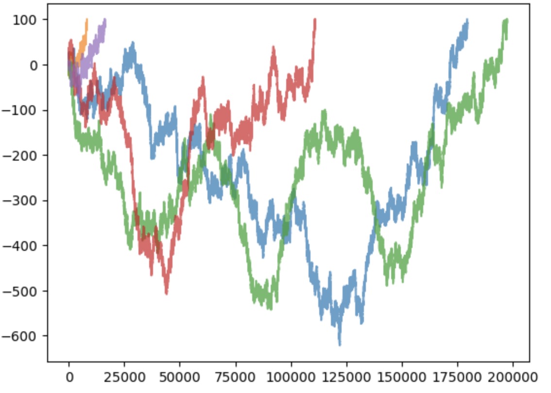
Example: The Drunkard’s Walk#

The following code models a random walker that takes random steps until it reaches some predefined position called “home”. This problem is often known as the drunkard’s walk, as it models a drunk person rambling until they get home and pass out.

We implement it in an object-oriented manner.

import numpy as np
import matplotlib.pyplot as plt


class DrunkardsWalk:
    def __init__(self, home):
        self.x = 0
        self.home = home
        self.history = [0]

    @property
    def position(self):
        return self.x

    @property
    def steps(self):
        return len(self.history)

    def is_at_home(self):
        return self.position == self.home

    def step(self):
        self.x += 2 * np.random.randint(2) - 1
        self.history.append(self.x)

    def walk_home(self):
        while not self.is_at_home():
            self.step()
        return self.steps

    def plot(self):
        plt.plot(range(self.steps), self.history, alpha=0.7)

for walker in range(5):
    drunkard = DrunkardsWalk(100)
    drunkard.walk_home()
    drunkard.plot()

plt.show()

Let us profile this code. In Python, a standard package for profiling is cProfile, which should come pre-packaged with Python installation.

import cProfile
np.random.seed(100122)
cProfile.run('DrunkardsWalk(100).walk_home()')

         4310769 function calls in 5.249 seconds

   Ordered by: standard name

   ncalls  tottime  percall  cumtime  percall filename:lineno(function)
   862153    0.129    0.000    0.129    0.000 1323739505.py:11(position)
        1    0.000    0.000    0.000    0.000 1323739505.py:15(steps)
   862153    0.341    0.000    0.470    0.000 1323739505.py:19(is_at_home)
   862152    0.889    0.000    4.286    0.000 1323739505.py:22(step)
        1    0.464    0.464    5.219    5.219 1323739505.py:26(walk_home)
        1    0.000    0.000    0.000    0.000 1323739505.py:6(__init__)
        1    0.030    0.030    5.249    5.249 <string>:1(<module>)
        1    0.000    0.000    5.249    5.249 {built-in method builtins.exec}
        1    0.000    0.000    0.000    0.000 {built-in method builtins.len}
   862152    0.120    0.000    0.120    0.000 {method 'append' of 'list' objects}
        1    0.000    0.000    0.000    0.000 {method 'disable' of '_lsprof.Profiler' objects}
   862152    3.276    0.000    3.276    0.000 {method 'randint' of 'numpy.random.mtrand.RandomState' objects}

The output from cProfile shows the time used by the different functions of the program. For each function, a row is printed. The name of the function is shown on the right-most side. The other columns show different information

ncalls: The number of times the function is called
tottime: Time spent inside the function without sub-functions it calls
cumtime: Time spent inside the function and inside functions it calls
per call: The time divided by the number of calls

To identify which parts of the code are slowest, we must look at the tottime column and find the largest number. Here the three largest are:

randint() with 3.276 seconds.
step() with 0.889 seconds.
walk_home() with 0.464 seconds.

At the top, it says the total time of execution is 5.249 seconds, so randint() uses over half of the execution time. An idea to optimize this code here could be to vectorize with NumPy. For example, we could create a 100-long array with 2 * np.random.randint(0, 2, 100) - 1.

Note also that there are some rows to functions that are technical, such as method 'disable' of '_lsprof.Profiler' objects, which can be ignored.

More on cProfile#

The cProfile package is a good tool for performing function profiling in Python. This means it explores how much time different functions spend. Instead of just writing out a big table, we can use the pstats package (“profiling stats”). Read more about cProfile and pstats on the official Python documentation here.

Line Profiling#

An alternative to function profiling with cProfile is to line profile. This means it divides the time used by the program into each separate line. The benefit of line profiling is that it does not just tells us which function is slow but exactly which lines inside a function are slow.

The line_profiler package can be used to do line profiling in Python. This needs to be installed and in Anaconda it can be done by writing:

Anaconda Python: conda install line_profiler

Another option is to install it using pip:

Other Pythons: pip3 install line_profiler

To use line_profiler inside a notebook, we need to load it as an external tool

%load_ext line_profiler

lpres = %lprun -r -f DrunkardsWalk.step -f DrunkardsWalk.walk_home DrunkardsWalk(100).walk_home()

Here we are telling line_profile to run the statement DrunkardWalk(100).walk_home() and analyze the performance of the two explicitly mentioned functions. The output pop up in a separate window:

Timer unit: 1e-06 s

Total time: 3.18336 s
File: <ipython-input-75-b157087bcb36>
Function: step at line 21

Line #      Hits         Time  Per Hit   % Time  Line Contents
==============================================================
    21                                               def step(self):
    22   1366246    2600136.0      1.9     81.7          self.x += 2*np.random.randint(2) - 1
    23   1366246     583225.0      0.4     18.3          self.history.append(self.x)

Total time: 5.77839 s
File: <ipython-input-75-b157087bcb36>
Function: walk_home at line 25

Line #      Hits         Time  Per Hit   % Time  Line Contents
==============================================================
    25                                               def walk_home(self):
    26   1366247    1015881.0      0.7     17.6          while not self.is_at_home():
    27   1366246    4762509.0      3.5     82.4              self.step()
    28         1          3.0      3.0      0.0          return self.steps

So we can see that line 22, where we increment the position, takes up 81.7% of the time it takes to use the step() method. As mentioned, vectorizing with NumPy might speed this up. Appending the elements to the history takes 20% of the time, which is also considerable. Perhaps it would be better to initialize an empty array and then update the elements?

Memory optimization#

So far, we have focused on optimizing concerning speed. Now, we turn to memory optimization. Specifically, we will explore how to optimize looping through a sequence with generators. A generator is an object that can be looped over similarly to lists, the difference being that generators do not store their content in memory. There are two main ways of defining a generator. The first way is by using a generator expression, which is similar to list comprehension but uses parenthesis instead of brackets.

iter_gen = (2 * i for i in range(1, 5))  # Generator
iter_list = [2 * i for i in range(1, 5)]  # List

Both of these can be iterated by using a for-loop.

for i in iter_gen:
    print(i)

for i in iter_list:
    print(i)

The main difference is that the generator does not store the values in memory. This can be demonstrated by printing the two objects.

print(iter_gen)
print(iter_list)

<generator object <genexpr> at 0x7f57c7acbd80>
[2, 4, 6, 8]

Since the generator does not store its values in memory, we can save considerable space.

import sys

gen = (2 * i for i in range(1, 100_000))
list = [2 * i for i in range(1, 100_000)]

print("gen uses", sys.getsizeof(gen), "bytes.")
print("list uses", sys.getsizeof(list), "bytes.")

gen uses 104 bytes.
list uses 800984 bytes.

The second way of defining a generator is by using a generator function.

def generator():
    for i in range(1, 5):
        yield 2 * i


for i in generator():
    print(i)

This is equivalent to the generator expression (2 * i for i in range(1, 5)). The generator seems like a regular function, only with yield instead of return. However, this behaves quite differently from a function. For each iterate in the for-loop, a function next() is called behind the scenes.

gen = generator()

for _ in range(1, 5):
    i = next(gen)
    print(i)

The line i = next(gen) executes lines in the function generator() until it reaches the yield-statement, then returns whatever is after the statement. The generator remembers what state it was in, so when next(gen) is called again, it continues where it stopped last time. The yield statement acts as both an entry and exit point.

Generators can be useful in several examples, such as dealing with large lists or files. It is, however, important to note that generators can be slower to evaluate than their list counterparts. So if memory is not an issue, generators should be avoided.

The Rules of Optimization#

We have discussed that if one wants to optimize, one should do so after getting the code to work correctly and elegantly. Even then, one should weigh the pros and cons and see if it is necessary.

If we start optimizing, we should also first get a proper handle on the bottlenecks of the program and focus on those, leaving the rest of the code alone.

This is summarized by what is called the rules of optimization

The first rule of optimization: Do not do it.
The second rule of optimization: Do not do it… yet.
The third rule of optimization: Profile before optimizing!

The root of all evil#

A famous quote in programming is called the root of all evil, and was made by Donald Knuth:

Programmers waste enormous amounts of time thinking about, or worrying about, the speed of noncritical parts of their programs, and these attempts at efficiency actually have a strong negative impact when debugging and maintenance are considered. We should forget about small efficiencies, say about 97% of the time: premature optimization is the root of all evil. Yet we should not pass up our opportunities in that critical 3%.”

The quote is often shortened to “premature optimization is the root of all evil”, which also summarizes the rule we started with: First, make it work, then, make it elegant, and lastly, make it fast. If we start optimizing while solving the problem for the first time, we are prematurely optimizing.

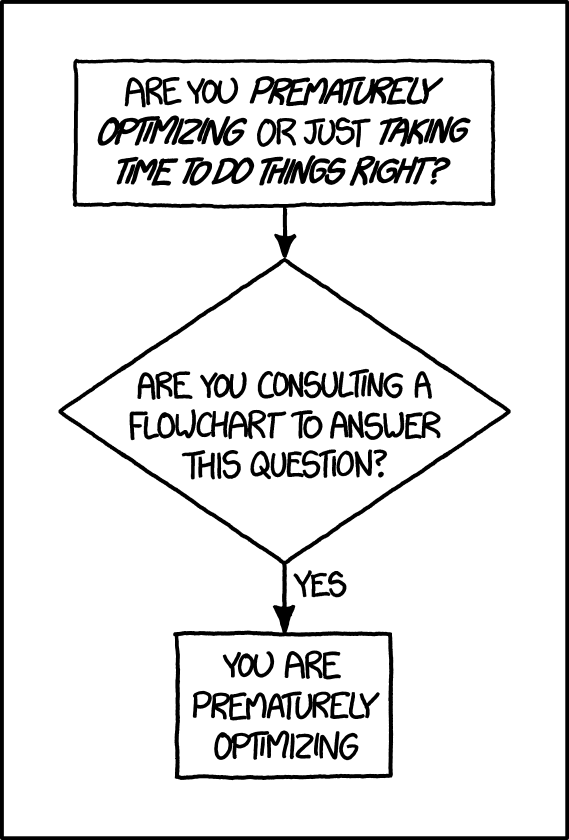
xkcd1691 — Fig. 61 **Source:** XKCD #1691#

There is a time and a place for optimization. When appropriate, it should be done in a structured, systematic manner.

Some take quotes like “premature optimization is the root of all evil” too much to heart and forgo optimization altogether. However, this is also far from ideal, which the full quote addresses! While some people use the quote to justify laziness and bad practices, others lose the bigger picture of making the code work first. The main takeaway is to have a balance.