Activation times from the eikonal equation

The eikonal equation gives the time \(t_a\) at which a wavefront, travelling with conduction velocity \(v_l\) along the fibres \(f\) and \(v_t\), \(v_n\) across them, reaches every point:

\[ \sqrt{\nabla t_a^T V \nabla t_a} = 1, \qquad V = v_l^2 f f^T + v_t^2 s s^T + v_n^2 n n^T, \]

with \(t_a = t_0\) on the sources. beat.eikonal solves it at the vertices of the mesh with the Fast Iterative Method [FKW13, JW08], a C kernel compiled on first use (and cached), on any number of MPI ranks. It is the cheap part of the reaction-eikonal model [NCP+17] (see the wedge demos), and is useful on its own, e.g. to build activation maps for electromechanics or to fit activation sequences.

import time

from mpi4py import MPI

import dolfinx
import matplotlib.pyplot as plt
import numpy as np
import scifem

import beat
from beat.eikonal import EikonalSolver, Source, solve_eikonal

comm = MPI.COMM_WORLD

A point-like source in anisotropic tissue

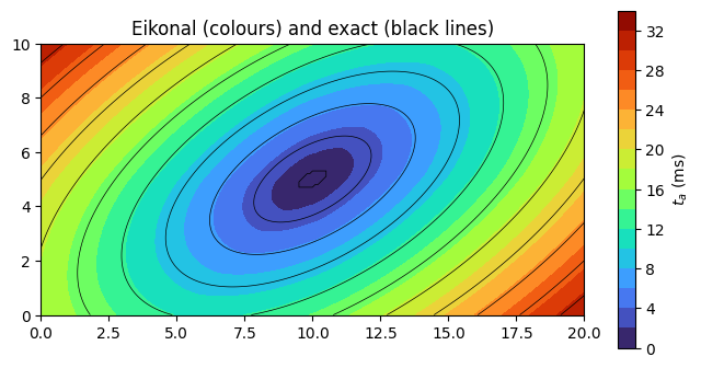
With constant \(V\) the exact solution from a source ball \(\|x - x_0\|_{V^{-1}} \le \rho\) is \(t_a = \max(0, \|x - x_0\|_{V^{-1}} - \rho)\), an ellipse stretched along the fibres. We use \(v_l = 0.6\) mm/ms, \(v_t = 0.3\) mm/ms and fibres at 30 degrees on a 20 x 10 mm sheet.

vl, vt = 0.6, 0.3
theta = np.deg2rad(30.0)
f = np.array([np.cos(theta), np.sin(theta)])
s = np.array([-np.sin(theta), np.cos(theta)])
x0, rho = np.array([10.0, 5.0]), 1.0
Vinv = np.eye(2) / vt**2 + (1 / vl**2 - 1 / vt**2) * np.outer(f, f)


def distance(x):
    d = x[:2] - x0[:, None]
    return np.sqrt(np.einsum("in,ij,jn->n", d, Vinv, d))


for h in (0.5, 0.25, 0.125):
    mesh = dolfinx.mesh.create_rectangle(
        comm, [[0.0, 0.0], [20.0, 10.0]], [round(20 / h), round(10 / h)],
    )
    fibers = (dolfinx.fem.Constant(mesh, f), dolfinx.fem.Constant(mesh, s))
    t_a = solve_eikonal(mesh, (vl, vt), fibers, [Source(lambda x: distance(x) <= rho + 1e-10)])
    exact = dolfinx.fem.Function(t_a.function_space)
    exact.interpolate(lambda x: np.maximum(0.0, distance(x) - rho))
    n = t_a.function_space.dofmap.index_map.size_local
    err = comm.allreduce(np.abs(t_a.x.array[:n] - exact.x.array[:n]).max(), op=MPI.MAX)
    if comm.rank == 0:
        print(f"h = {h:5.3f} mm: max error {err:.3f} ms")

h = 0.500 mm: max error 1.725 ms
h = 0.250 mm: max error 0.625 ms
h = 0.125 mm: max error 0.280 ms

The error decreases roughly linearly with the mesh size, as expected for this first-order method.

grid_x, grid_y = np.meshgrid(np.linspace(0, 20, 201), np.linspace(0, 10, 101))
points = np.column_stack([grid_x.ravel(), grid_y.ravel()])
values = scifem.evaluate_function(t_a, points).reshape(grid_x.shape)
if comm.rank == 0:
    fig, ax = plt.subplots(figsize=(8, 4))
    c = ax.contourf(grid_x, grid_y, values, levels=20, cmap="turbo")
    ax.contour(
        grid_x, grid_y, np.maximum(0, distance(points.T).reshape(grid_x.shape) - rho),
        levels=10, colors="k", linewidths=0.5,
    )
    fig.colorbar(c, label="$t_a$ (ms)")
    ax.set_aspect("equal")
    ax.set_title("Eikonal (colours) and exact (black lines)")
    fig.savefig("eikonal_point_source.png")

Colliding fronts

Sources can start at different times. Two plane waves, from the left edge at \(t = 0\) and from the right edge at \(t = 5\) ms, collide where \(x / v_l = 5 + (20 - x) / v_l\), i.e. at \(x = 11.5\) mm; the eikonal solution is exact for plane waves.

mesh = dolfinx.mesh.create_rectangle(comm, [[0.0, 0.0], [20.0, 10.0]], [40, 20])
fibers = (dolfinx.fem.Constant(mesh, np.array([1.0, 0.0])), dolfinx.fem.Constant(mesh, np.array([0.0, 1.0])))
t_a = solve_eikonal(
    mesh,
    (vl, vt),
    fibers,
    [Source(lambda x: np.isclose(x[0], 0.0), 0.0), Source(lambda x: np.isclose(x[0], 20.0), 5.0)],
)
line = np.column_stack([np.linspace(0, 20, 81), np.full(81, 5.0)])
values = scifem.evaluate_function(t_a, line).ravel()
if comm.rank == 0:
    print(f"latest activation at x = {line[np.argmax(values), 0]:.2f} mm (expected 11.5 mm)")

latest activation at x = 11.50 mm (expected 11.5 mm)

The wedge of Neic et al. (2017)

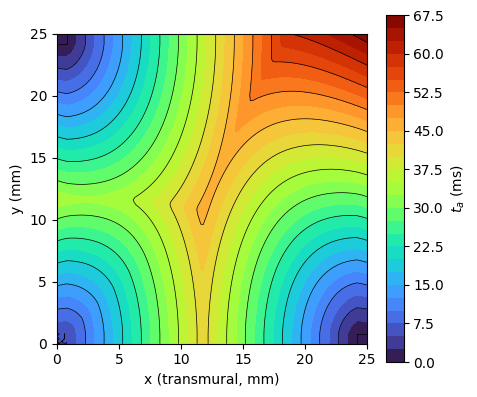
A 25 x 25 x 5 mm piece of ventricular wall with fibres rotating by 120 degrees across it, and three stimuli: S1 and S3 at \(t = 0\) and S2 at \(t = 5\) ms. get_3D_wedge_geometry returns the stimulus regions as cell tags, which Source accepts directly. An EikonalSolver sets up the mesh and metric once and can then be reused for many source sets.

wedge = beat.geometry.get_3D_wedge_geometry(comm, dx=0.4)
geo = wedge.geometry
solver = EikonalSolver(geo.mesh, (0.6, 0.3, 0.3), (geo.f0, geo.s0, geo.n0))
sources = [Source((wedge.cell_tags, tag), t0) for tag, t0 in wedge.stimuli.values()]
start = time.perf_counter()
t_a = solver.solve(sources)
elapsed = time.perf_counter() - start
if comm.rank == 0:
    print(f"wedge, {solver.V.dofmap.index_map.size_global} vertices: {elapsed:.2f} s, {solver.stats}")

grid_x, grid_y = np.meshgrid(np.linspace(0, 25, 126), np.linspace(0, 25, 126))
points = np.column_stack([grid_x.ravel(), grid_y.ravel(), np.full(grid_x.size, 2.5)])
values = scifem.evaluate_function(t_a, points).reshape(grid_x.shape)
if comm.rank == 0:
    fig, ax = plt.subplots(figsize=(5, 4.5))
    c = ax.contourf(grid_x, grid_y, values, levels=np.arange(0, 70, 2.5), cmap="turbo")
    ax.contour(grid_x, grid_y, values, levels=np.arange(0, 70, 5), colors="k", linewidths=0.5)
    fig.colorbar(c, label="$t_a$ (ms)")
    ax.set_xlabel("x (transmural, mm)")
    ax.set_ylabel("y (mm)")
    ax.set_aspect("equal")
    fig.savefig("eikonal_wedge.png")

wedge, 51597 vertices: 0.36 s, {'rounds': 1, 'passes': 81, 'updates': 296123}

Run the demo with e.g. mpirun -n 4 python eikonal.py; the result does not depend on the number of ranks. Pass openmp=True (and num_threads) to EikonalSolver to also use threads within each rank. Quadrilateral and hexahedral meshes, and meshes with higher-order geometry, work the same way (only the vertices are used).