Spiral wave in a 2D sheet of human ventricular tissue#
Spiral waves (also called rotors, or re-entrant waves) are self-sustained rotating waves of electrical activity that are believed to underlie many dangerous cardiac arrhythmias, such as ventricular tachycardia and, once they break up into many smaller waves, ventricular fibrillation. In this demo we initiate a single spiral wave in a 2D square sheet of human ventricular tissue, using the ten Tusscher–Panfilov 2006 (TP06) cell model [tTP06, tTNNP04], and follow its rotation centre (the spiral tip) over time.
The setup follows the 2D tissue simulations of ten Tusscher and Panfilov [tTP06, tTNNP04]: isotropic tissue, the default (epicardial) TP06 parameters, and a classical cross-field S1–S2 stimulation protocol to start the spiral. The spiral wave breakup demo uses the same setup with one of the parameter sets from [tTP06] that makes the spiral unstable.
We solve the monodomain model
with \(M\) and \(I_{stim}\) expressed per unit membrane area (i.e. already divided by the surface to
volume ratio \(\chi\)), using beat.MonodomainSplittingSolver. See the
mathematical background page for the notation, and the
FitzHugh–Nagumo demo for a step-by-step introduction to the beat API.
Note: simulating the spiral for 2 s takes about 20 minutes on a single core, which is too long
for building the documentation. We therefore only simulate the first 10 ms by default, and show
results from a precomputed simulation with end_time = 2000.0 at the end of the demo.
comm = MPI.COMM_WORLD
results_folder = Path("results-spiral-wave")
results_folder.mkdir(exist_ok=True)
Parameters#
Human ventricular tissue has a long action potential (about 300 ms) and a fast conduction velocity (about 70 cm/s), so the wavelength of a wave (conduction velocity times action potential duration) is about 20 cm. A spiral wave therefore needs a fairly large piece of tissue to fit in. ten Tusscher et al. used a \(12 \times 12\) cm sheet [tTNNP04] and a \(25 \times 25\) cm sheet [tTP06]. Here we use a \(10 \times 10\) cm square, which is large enough for the spiral to survive for the 2 s we simulate.
The papers use a grid spacing of 0.2–0.25 mm. To keep the run time down we use a mesh size of
0.5 mm, which with linear elements gives a conduction velocity within a couple of percent of the
one at 0.25 mm. Lower h (and dt) if you
want to match the papers more closely, and run the demo in parallel with e.g. mpirun -n 8 python spiral_wave.py.
L = 100.0  # Side length of the square (mm)
h = 0.5  # Mesh size (mm)
dt = 0.05  # Time step (ms)
end_time = 10.0  # Simulation time (ms). Set to 2000.0 to reproduce the results below
t_S2 = 340.0  # Start time of the S2 stimulus (ms)
Cell model#
We use the epicardial version of the TP06 model, and generate code for it with gotranx, using
the generalized Rush–Larsen scheme for the gating variables, just as in the original paper.
model_path = Path("tentusscher_panfilov_2006_epi_cell.py")
if not model_path.is_file():
    here = Path.cwd()
    cell_ode = gotranx.load_ode(
        here
        / ".."
        / "odes"
        / "tentusscher_panfilov_2006"
        / "tentusscher_panfilov_2006_epi_cell.ode",
    )
    code = gotranx.cli.gotran2py.get_code(
        cell_ode,
        scheme=[gotranx.schemes.Scheme.generalized_rush_larsen],
    )
    model_path.write_text(code)
import tentusscher_panfilov_2006_epi_cell as model
The default parameters in the .ode file are the default TP06 parameters (the “slope 1.1” set in
[tTP06]). We switch off the stimulus current in the cell model, since the
stimuli are applied through the PDE instead, and start every cell from the resting state.
parameters = model.init_parameter_values(stim_amplitude=0.0)
init_states = model.init_state_values()
v_index = model.state_index("V")
Geometry and stimulus#
We create a square mesh \([0, L]^2\) (in mm), with triangular elements.
N = int(round(L / h))
mesh = dolfinx.mesh.create_rectangle(
    comm,
    [[0.0, 0.0], [L, L]],
    [N, N],
    dolfinx.mesh.CellType.triangle,
)
To start a spiral wave we use a cross-field S1–S2 protocol:
S1: a stimulus along the left edge (\(x \leq 1\) mm) at \(t = 0\), starting a planar wave that travels to the right.
S2: a stimulus in the lower left quadrant (\(x \leq L/2\), \(y \leq L/2\)) at \(t = t_{S2}\), after the S1 wave has passed. At that point, the tissue behind the S1 wave (to the left) has recovered, while the tissue to the right is still refractory. The S2 wave can therefore only propagate upwards and to the left, and the free end of its wavefront at the centre of the square curls around into a spiral.
The timing of the S2 stimulus is important: too early and the S2 wave cannot propagate at all
(try t_S2 = 300), and much later the whole square has recovered so that the S2 wave also
propagates to the right, and no spiral forms. We found \(t_{S2} = 340\) ms by trial and error.
Both stimuli use the same cell tags, with different markers.
S1_marker = 1
S2_marker = 2
tol = 1e-8


def S1_subdomain(x):
    return x[0] <= 1.0 + tol


def S2_subdomain(x):
    return np.logical_and(x[0] <= L / 2 + tol, x[1] <= L / 2 + tol)


tdim = mesh.topology.dim
S1_cells = dolfinx.mesh.locate_entities(mesh, tdim, S1_subdomain)
S2_cells = np.setdiff1d(dolfinx.mesh.locate_entities(mesh, tdim, S2_subdomain), S1_cells)
cells = np.concatenate([S1_cells, S2_cells])
values = np.concatenate(
    [np.full(len(S1_cells), S1_marker), np.full(len(S2_cells), S2_marker)],
).astype(np.int32)
order = np.argsort(cells)
stim_tags = dolfinx.mesh.meshtags(mesh, tdim, cells[order], values[order])
The surface to volume ratio \(\chi\) and the membrane capacitance \(C_m\)
chi = beat.units.ureg.Quantity(1400.0, "cm**-1")
C_m = beat.units.ureg.Quantity(1.0, "uF/cm**2").to("uF/mm**2").magnitude
and the two stimuli, lasting 2 ms (S1) and 5 ms (S2) as in [tTP06]. The amplitude of 50 000 µA/cm³ is comfortably above the excitation threshold.
time = dolfinx.fem.Constant(mesh, 0.0)
I_s = [
    beat.stimulation.define_stimulus(
        mesh=mesh,
        chi=chi,
        time=time,
        subdomain_data=stim_tags,
        marker=S1_marker,
        mesh_unit="mm",
        amplitude=50_000.0,
        start=0.0,
        duration=2.0,
    ),
    beat.stimulation.define_stimulus(
        mesh=mesh,
        chi=chi,
        time=time,
        subdomain_data=stim_tags,
        marker=S2_marker,
        mesh_unit="mm",
        amplitude=50_000.0,
        start=t_S2,
        duration=5.0,
    ),
]
Conductivity#
The tissue is isotropic, so the conductivity tensor \(M\) is a scalar. Dividing the monodomain equation by \(C_m\), we see that the diffusion coefficient of the tissue is \(D = M / C_m\).
ten Tusscher and Panfilov use \(D = 0.154\) mm²/ms, which gives a planar conduction velocity of 68 cm/s with their finite difference scheme [tTP06]. With the finite element and operator splitting scheme used here, the same \(D\) gives about 76 cm/s, even with a 0.25 mm mesh. Since the conduction velocity (and hence the wavelength) is what governs the dynamics of the spiral, we instead scale \(D\) to match the paper’s conduction velocity. Conduction velocity scales with \(\sqrt{D}\), so \(D = 0.154 \cdot (68 / 76)^2 \approx 0.122\) mm²/ms. We check the conduction velocity of the S1 wave further down.
D = 0.122  # mm^2 / ms
M = D * C_m
Solvers#
pde = beat.MonodomainModel(
    time=time,
    mesh=mesh,
    M=M,
    I_s=I_s,
    C_m=C_m,
    dx=I_s[0].dZ,
    params={
        "petsc_options": {
            "ksp_type": "cg",
            "pc_type": "hypre",
            "pc_hypre_type": "boomeramg",
        },
    },
)
ode = beat.odesolver.DolfinODESolver(
    v_ode=dolfinx.fem.Function(dolfinx.fem.functionspace(mesh, ("P", 1))),
    v_pde=pde.state,
    fun=model.generalized_rush_larsen,
    init_states=init_states,
    parameters=parameters,
    num_states=len(init_states),
    v_index=v_index,
)
solver = beat.MonodomainSplittingSolver(pde=pde, ode=ode)
v = solver.pde.v
Tracking the spiral tip#
The tip of a spiral wave is the point where the wavefront (where \(v\) is increasing) meets the waveback (where \(v\) is decreasing). Following [FK98], we locate it as the intersection of the iso-potential line \(v = V_{iso}\) and the line \(\partial v / \partial t = 0\).
With linear (P1) elements, both \(v - V_{iso}\) and the time difference \(v(t) - v(t - \Delta t_{tip})\) are linear on each triangle, so each of the two lines is a straight segment within a triangle, and the intersection can be computed exactly by solving a \(2\times2\) linear system in the local (barycentric) coordinates of the triangle. Close to the tip, the two lines are almost parallel, so they may cross several times within a few millimetres. We therefore merge all points that are closer than 1 cm, which is still much smaller than the distance between two separate spiral tips.
V_iso = -40.0  # mV
Vh = v.function_space
num_owned_cells = mesh.topology.index_map(tdim).size_local
cell_dofs = Vh.dofmap.list[:num_owned_cells]
dof_coords = Vh.tabulate_dof_coordinates()[:, :2]


def merge_points(points, radius=10.0):
    clusters: list[list[np.ndarray]] = []
    for p in points:
        for c in clusters:
            if np.linalg.norm(np.mean(c, axis=0) - p) < radius:
                c.append(p)
                break
        else:
            clusters.append([p])
    return np.array([np.mean(c, axis=0) for c in clusters]).reshape(-1, 2)


def find_tips(v_now, v_prev):
    a = v_now[cell_dofs] - V_iso
    b = (v_now - v_prev)[cell_dofs]
    # Triangles where both lines pass through
    candidates = (a.min(1) < 0) & (a.max(1) > 0) & (b.min(1) < 0) & (b.max(1) > 0)
    a, b = a[candidates], b[candidates]
    x = dof_coords[cell_dofs[candidates]]
    A = np.stack(
        [
            np.stack([a[:, 1] - a[:, 0], a[:, 2] - a[:, 0]], axis=-1),
            np.stack([b[:, 1] - b[:, 0], b[:, 2] - b[:, 0]], axis=-1),
        ],
        axis=1,
    )
    rhs = -np.stack([a[:, 0], b[:, 0]], axis=-1)
    regular = np.abs(np.linalg.det(A)) > 1e-14
    xi = np.zeros_like(rhs)
    xi[regular] = np.linalg.solve(A[regular], rhs[regular][..., None])[..., 0]
    inside = regular & (xi[:, 0] >= 0) & (xi[:, 1] >= 0) & (xi.sum(axis=1) <= 1)
    points = x[:, 0] + xi[:, :1] * (x[:, 1] - x[:, 0]) + xi[:, 1:] * (x[:, 2] - x[:, 0])
    all_points = np.vstack(comm.allgather(points[inside]))
    return merge_points(all_points)
Output#
We save \(v\) to a VTX file that can be opened in ParaView, record \(v\) at three probe points, and,
if pyvista is available, make an animation where the current tip position is shown in red.
vtx_file = results_folder / "spiral_wave.bp"
shutil.rmtree(vtx_file, ignore_errors=True)
vtx = dolfinx.io.VTXWriter(comm, vtx_file, [v], engine="BP4")

probes = np.array([[L / 4, L / 2], [3 * L / 4, L / 2], [0.9 * L, 0.9 * L]])

make_gif = pyvista is not None and comm.size == 1
if make_gif:
    pyvista.OFF_SCREEN = True
    plotter = pyvista.Plotter(window_size=[600, 600])
    grid = pyvista.UnstructuredGrid(*dolfinx.plot.vtk_mesh(Vh))
    grid.point_data["V"] = v.x.array
    grid.set_active_scalars("V")
    plotter.add_mesh(grid, cmap="viridis", clim=[-90.0, 40.0], lighting=False)
    plotter.view_xy()
    gif_file = Path("spiral_wave.gif")
    gif_file.unlink(missing_ok=True)
    plotter.open_gif(gif_file.as_posix())
Time stepping#
Every millisecond we evaluate the probes and look for spiral tips, using the potential from the previous millisecond to approximate the sign of \(\partial v / \partial t\). We start looking for tips shortly after the S2 stimulus.
probe_every = round(1.0 / dt)
frame_every = round(10.0 / dt)

probe_time_list: list[float] = []
probe_value_list: list[np.ndarray] = []
tip_list: list[list[float]] = []  # rows of (t, x, y)
v_prev = v.x.array.copy()

t = 0.0
i = 0
num_steps = round(end_time / dt)
while i <= num_steps:
    if i % probe_every == 0:
        probe_time_list.append(t)
        probe_value_list.append(scifem.evaluate_function(v, probes).ravel())
        current_tips = find_tips(v.x.array, v_prev) if t > t_S2 + 10 else np.zeros((0, 2))
        tip_list.extend([t, *p] for p in current_tips)
        v_prev[:] = v.x.array

    if i % frame_every == 0:
        vtx.write(t)
        if comm.rank == 0 and i % (100 * probe_every) == 0:
            print(f"t = {t:.0f} ms, number of tips: {len(current_tips)}")
        if make_gif:
            grid.point_data["V"] = v.x.array
            if len(current_tips) > 0:
                plotter.add_points(
                    np.hstack([current_tips, np.ones((len(current_tips), 1))]),
                    color="red",
                    point_size=12,
                    render_points_as_spheres=True,
                    name="tips",
                )
            else:
                plotter.remove_actor("tips")
            plotter.add_text(f"t = {t:.0f} ms", name="time", font_size=12)
            plotter.write_frame()

    solver.step((t, t + dt))
    i += 1
    t += dt

vtx.close()
if make_gif:
    plotter.close()
t = 0 ms, number of tips: 0
Results#
The analysis below needs a longer simulation than the default 10 ms (set end_time = 2000.0); the
figures at the end of the demo show the results from such a simulation.
First, we check the conduction velocity of the planar S1 wave from the time it passes the first two probes, which lie \(L/2\) apart on the line \(y = L/2\).
probe_times = np.array(probe_time_list)
probe_values = np.array(probe_value_list)
tips = np.array(tip_list).reshape(-1, 3)


def upstroke_times(trace, threshold=-40.0):
    crossing = (trace[:-1] < threshold) & (trace[1:] >= threshold)
    return probe_times[1:][crossing]


t1 = upstroke_times(probe_values[:, 0])
t2 = upstroke_times(probe_values[:, 1])
if len(t1) > 0 and len(t2) > 0 and comm.rank == 0:
    cv = (L / 2) / (t2[0] - t1[0])  # mm/ms = m/s
    print(f"Conduction velocity: {100 * cv:.1f} cm/s (paper: 68 cm/s)")
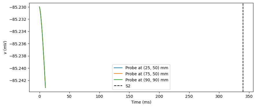
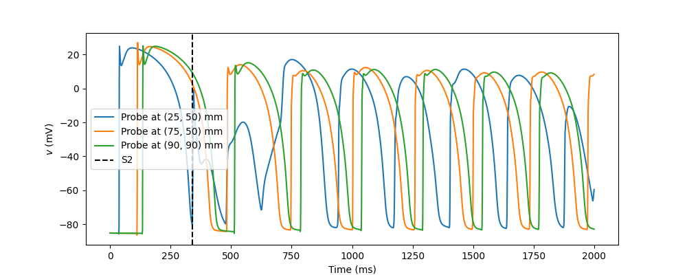
The spiral rotation period is the time between consecutive activations at a probe once the spiral has settled. We skip the first second, where the initial S1 and S2 waves still dominate.
fig, ax = plt.subplots(figsize=(10, 4))
for k, p in enumerate(probes):
    ax.plot(probe_times, probe_values[:, k], label=f"Probe at ({p[0]:.0f}, {p[1]:.0f}) mm")
ax.axvline(t_S2, color="k", linestyle="--", label="S2")
ax.set_xlabel("Time (ms)")
ax.set_ylabel("$v$ (mV)")
ax.legend()
fig.savefig("spiral_wave_probes.png")

period_list: list[float] = []
for k in range(len(probes)):
    activations = upstroke_times(probe_values[:, k])
    period_list.extend(np.diff(activations[activations > 1000.0]))
periods = np.array(period_list)
if len(periods) > 0 and comm.rank == 0:
    print(f"Spiral period: {periods.mean():.0f} ± {periods.std():.0f} ms")
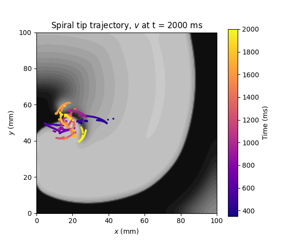
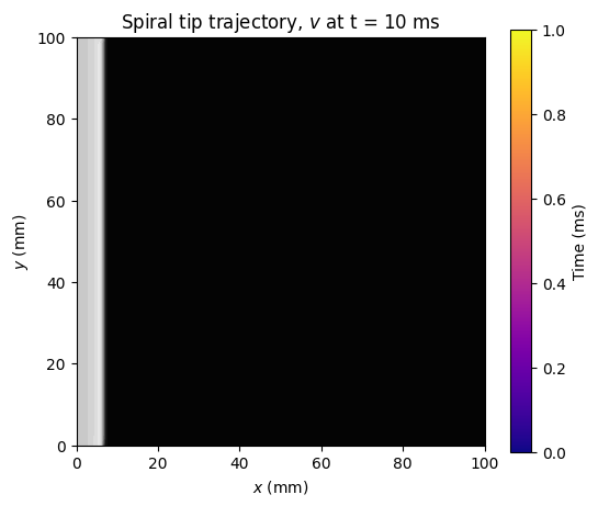
Finally, we plot the trajectory of the spiral tip, coloured by time, on top of the final potential. The spiral tip does not rotate around a fixed point, but meanders, tracing out a complex path that is several centimetres wide, as also observed by ten Tusscher et al. [tTNNP04].
nloc = Vh.dofmap.index_map.size_local
gathered = comm.gather(np.hstack([dof_coords[:nloc], v.x.array[:nloc, None]]), root=0)
if comm.rank == 0:
    assert gathered is not None
    final = np.vstack(gathered)
    fig, ax = plt.subplots(figsize=(6, 5))
    levels = np.linspace(-90, 40, 27)
    ax.tricontourf(final[:, 0], final[:, 1], final[:, 2], levels=levels, cmap="gray")
    sc = ax.scatter(tips[:, 1], tips[:, 2], c=tips[:, 0], s=3, cmap="plasma")
    fig.colorbar(sc, ax=ax, label="Time (ms)")
    ax.set_xlim(0, L)
    ax.set_ylim(0, L)
    ax.set_aspect("equal")
    ax.set_xlabel("$x$ (mm)")
    ax.set_ylabel("$y$ (mm)")
    ax.set_title(f"Spiral tip trajectory, $v$ at t = {end_time:.0f} ms")
    fig.savefig("spiral_wave_tip.png")
Precomputed results#
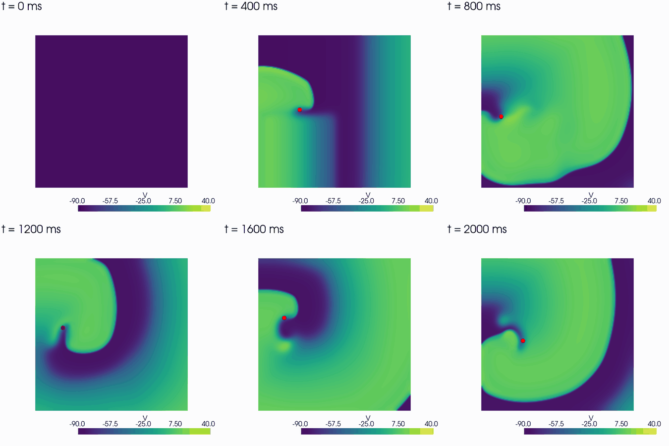
Here are the results from a simulation with end_time = 2000.0. The animation shows the S1 wave
travelling to the right, the S2 stimulus in the lower left quadrant, and the spiral wave that
forms at the end of the S2 wavefront, with the spiral tip in red.
The S1 wave travels at 66.7 cm/s, close to the 68 cm/s in [tTP06]. Once the spiral has settled, it activates the probes with a period of \(241 \pm 8\) ms. ten Tusscher et al. report a period of \(264.7 \pm 10.5\) ms on a \(12 \times 12\) cm sheet [tTNNP04], i.e. in the same range, given our slightly smaller domain and different numerical scheme.
The trajectory of the spiral tip shows that it does not rotate around a fixed point, but meanders over a region several centimetres wide.