The reaction-eikonal model: extracellular potentials and electrograms in a ventricular wedge

This demo reproduces Fig. 7 of Neic et al. [NCP+17]: extracellular potentials \(\phi_e\) and the electrogram at the electrode \(P_E\) for the reaction-diffusion (R-D) model and the reaction-eikonal models R-E\(^+\) and R-E\(^-\) on the wedge of the activation demo, now immersed in a 1 S/m bath.

As in the paper, all three models are pseudo-bidomain models (Section 8.4 of the mathematical background): the transmembrane potential \(v\) comes from a monodomain (or R-E) model whose conductivity is augmented in a thin layer along the tissue-bath interface to mimic bath loading [BP11], and \(\phi_e\) in tissue and bath is recovered from \(v\) by one elliptic solve whenever it is needed. Electrograms at a fixed electrode are computed from a precomputed lead field, at the cost of one integral per time step.

The live part runs R-E\(^-\) on the 400 µm wedge for 40 ms; the full results (100 µm R-D, R-E\(^+\), R-E\(^-\) and 400 µm R-E\(^+\) for 400 ms, from scripts/reaction_eikonal_wedge*.py) are shown at the end.

from pathlib import Path

from mpi4py import MPI

import dolfinx
import gotranx
import matplotlib.pyplot as plt
import numpy as np

import beat
from beat.eikonal import Source, solve_eikonal
from beat.pseudo_bidomain import LeadFieldElectrodes, VolumeConductor
from beat.reaction_eikonal import ExponentialFoot, FootCurrentODESolver
from beat.utils import PointEvaluator

comm = MPI.COMM_WORLD
dx = 0.4  # mm
end_time = 40.0  # ms
dt = 0.02  # ms

The wedge and its bath

get_3D_wedge_bath_geometry builds a box of bath around the wedge on the same grid, so the tissue part of the bath mesh has exactly the wedge’s vertices and cells and \(v\) moves between the two meshes without interpolation error. The paper does not give the size of the bath; we use 1 mm on every side (the bath-loading effect saturates at about that thickness [BP11], and a thicker bath does not fit in memory at 100 µm on the ~32 GB machine used here, about 21 GB free).

wedge = beat.geometry.get_3D_wedge_geometry(comm, dx=dx)
geo = wedge.geometry
mesh = geo.mesh
V = dolfinx.fem.functionspace(mesh, ("P", 1))
layers = beat.geometry.wedge_layer_markers(V)
bath = beat.geometry.get_3D_wedge_bath_geometry(comm, dx=dx, margin=1.0)
g = beat.conductivities.default_conductivities("Neic2017_wedge_bath")


def S(name):
    return g[name].to("S/m").magnitude


assert bath.geometry.f0 is not None
sigma_i_bath = beat.conductivities.conductivity_tensor(S("g_il"), S("g_it"), bath.geometry.f0)
sigma_e_bath = beat.conductivities.conductivity_tensor(S("g_el"), S("g_et"), bath.geometry.f0)
markers = beat.geometry.WEDGE_BATH_MARKERS
conductor = VolumeConductor(
    bath.geometry.mesh, bath.cell_tags, markers["TISSUE"], markers["BATH"], sigma_i_bath, sigma_e_bath, S("g_b"),
)
if comm.rank == 0:
    print(f"bath margins {bath.margins} mm, {bath.geometry.mesh.topology.index_map(0).size_global} vertices")

bath margins [1.20967742 1.20967742 1.25      ] mm, 90459 vertices

R-E\(^-\) with an electrogram at \(P_E\)

The ten Tusscher-Panfilov cell models and the eikonal activation time are set up as in the activation demo. R-E\(^-\) has no diffusion, so the augmented conductivity does not enter here; it does enter R-D and R-E\(^+\) (see the scripts).

ode_dir = Path.cwd().parent / "odes" / "tentusscher_panfilov_2006"
cell_models = {}
for layer, name in {"EPI": "epi", "M": "M", "ENDO": "endo"}.items():
    code = gotranx.cli.gotran2py.get_code(
        gotranx.load_ode(ode_dir / f"tentusscher_panfilov_2006_{name}_cell.ode"),
        scheme=[gotranx.schemes.Scheme.generalized_rush_larsen],
    )
    namespace: dict = {}
    exec(code, namespace)
    cell_models[beat.geometry.WEDGE_LAYERS[layer]] = namespace
init = {k: m["init_state_values"]() for k, m in cell_models.items()}
cells = beat.odesolver.DolfinMultiODESolver(
    v_ode=dolfinx.fem.Function(V),
    v_pde=dolfinx.fem.Function(V),
    markers=layers,
    init_states=init,
    parameters={k: m["init_parameter_values"](stim_amplitude=0.0) for k, m in cell_models.items()},
    fun={k: m["generalized_rush_larsen"] for k, m in cell_models.items()},
    num_states={k: len(v) for k, v in init.items()},
    v_index={k: m["state_index"]("V") for k, m in cell_models.items()},
)
cv = (0.594, 0.324, 0.324)  # mm/ms, from scripts/reaction_eikonal_cv.json
sources = [Source((wedge.cell_tags, tag), t0) for tag, t0 in wedge.stimuli.values()]
t_a = solve_eikonal(mesh, cv, (geo.f0, geo.s0, geo.n0), sources)
solver = beat.SplittingSolver(pde=None, ode=FootCurrentODESolver(cells, t_a, ExponentialFoot()))
v = solver.v

assert geo.f0 is not None
sigma_i = beat.conductivities.conductivity_tensor(S("g_il"), S("g_it"), geo.f0)
electrodes = LeadFieldElectrodes(conductor, v, sigma_i, {"P_E": wedge.electrode})
trace_t, trace = [0.0], [electrodes()["P_E"]]
t = 0.0
while t < end_time - 1e-9:
    solver.step((t, t + dt))
    t += dt
    if round(t / dt) % 5 == 0:
        trace_t.append(t)
        trace.append(electrodes()["P_E"])

2026-11-13 14:20:10 [info     ] Load ode /__w/fenicsx-beat/fenicsx-beat/odes/tentusscher_panfilov_2006/tentusscher_panfilov_2006_epi_cell.ode

2026-11-13 14:20:11 [warning  ] Dropping a guard whose replacement failed its numeric check value=0 var=Ca_i

2026-11-13 14:20:11 [warning  ] Dropping a guard whose replacement failed its numeric check value=0 var=K_i

2026-11-13 14:20:11 [warning  ] Dropping a guard whose replacement failed its numeric check value=0 var=Na_i

2026-11-13 14:20:11 [info     ] Num states 19                 

2026-11-13 14:20:11 [info     ] Num parameters 53             

2026-11-13 14:20:14 [info     ] Load ode /__w/fenicsx-beat/fenicsx-beat/odes/tentusscher_panfilov_2006/tentusscher_panfilov_2006_M_cell.ode

2026-11-13 14:20:15 [warning  ] Dropping a guard whose replacement failed its numeric check value=0 var=Ca_i

2026-11-13 14:20:15 [warning  ] Dropping a guard whose replacement failed its numeric check value=0 var=K_i

2026-11-13 14:20:15 [warning  ] Dropping a guard whose replacement failed its numeric check value=0 var=Na_i

2026-11-13 14:20:16 [info     ] Num states 19                 

2026-11-13 14:20:16 [info     ] Num parameters 53             

2026-11-13 14:20:19 [info     ] Load ode /__w/fenicsx-beat/fenicsx-beat/odes/tentusscher_panfilov_2006/tentusscher_panfilov_2006_endo_cell.ode

2026-11-13 14:20:19 [warning  ] Dropping a guard whose replacement failed its numeric check value=0 var=Ca_i

2026-11-13 14:20:19 [warning  ] Dropping a guard whose replacement failed its numeric check value=0 var=K_i

2026-11-13 14:20:19 [warning  ] Dropping a guard whose replacement failed its numeric check value=0 var=Na_i

2026-11-13 14:20:20 [info     ] Num states 19                 

2026-11-13 14:20:20 [info     ] Num parameters 53             

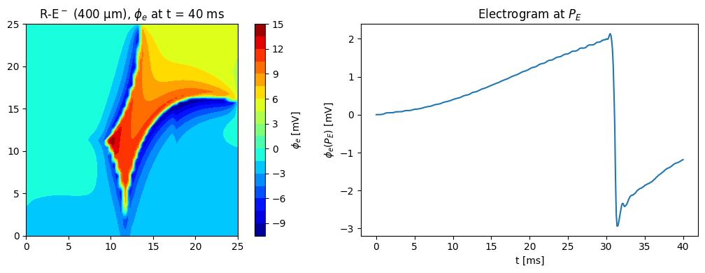
The extracellular potential at \(t = 40\) ms on the mid-plane \(z = 2.5\) mm, next to the electrogram so far:

phi_e = conductor.solve(v)
gx, gy = np.meshgrid(np.linspace(0, 25, 101), np.linspace(0, 25, 101))
points = np.column_stack([gx.ravel(), gy.ravel(), np.full(gx.size, 2.5)])
phi_grid = PointEvaluator(bath.geometry.mesh, points)(phi_e).reshape(gx.shape)
if comm.rank == 0:
    fig, (ax0, ax1) = plt.subplots(1, 2, figsize=(11, 4))
    cs = ax0.contourf(gx, gy, phi_grid, levels=21, cmap="jet")
    fig.colorbar(cs, ax=ax0, label=r"$\phi_e$ [mV]")
    ax0.set_aspect("equal")
    ax0.set_title(rf"R-E$^-$ (400 µm), $\phi_e$ at t = {end_time:g} ms")
    ax1.plot(trace_t, trace)
    ax1.set_xlabel("t [ms]")
    ax1.set_ylabel(r"$\phi_e(P_E)$ [mV]")
    ax1.set_title("Electrogram at $P_E$")
    fig.tight_layout()
    plt.show()

Precomputed results

The figure below was computed with the scripts in scripts/ on 16 MPI ranks (see their docstrings): the lead field of \(P_E\) (reaction_eikonal_wedge_leadfield.py), the bath-loaded runs with electrograms and snapshots of \(v\) at 40 and 320 ms (reaction_eikonal_wedge.py), and \(\phi_e\) for each snapshot (reaction_eikonal_wedge_phie.py).

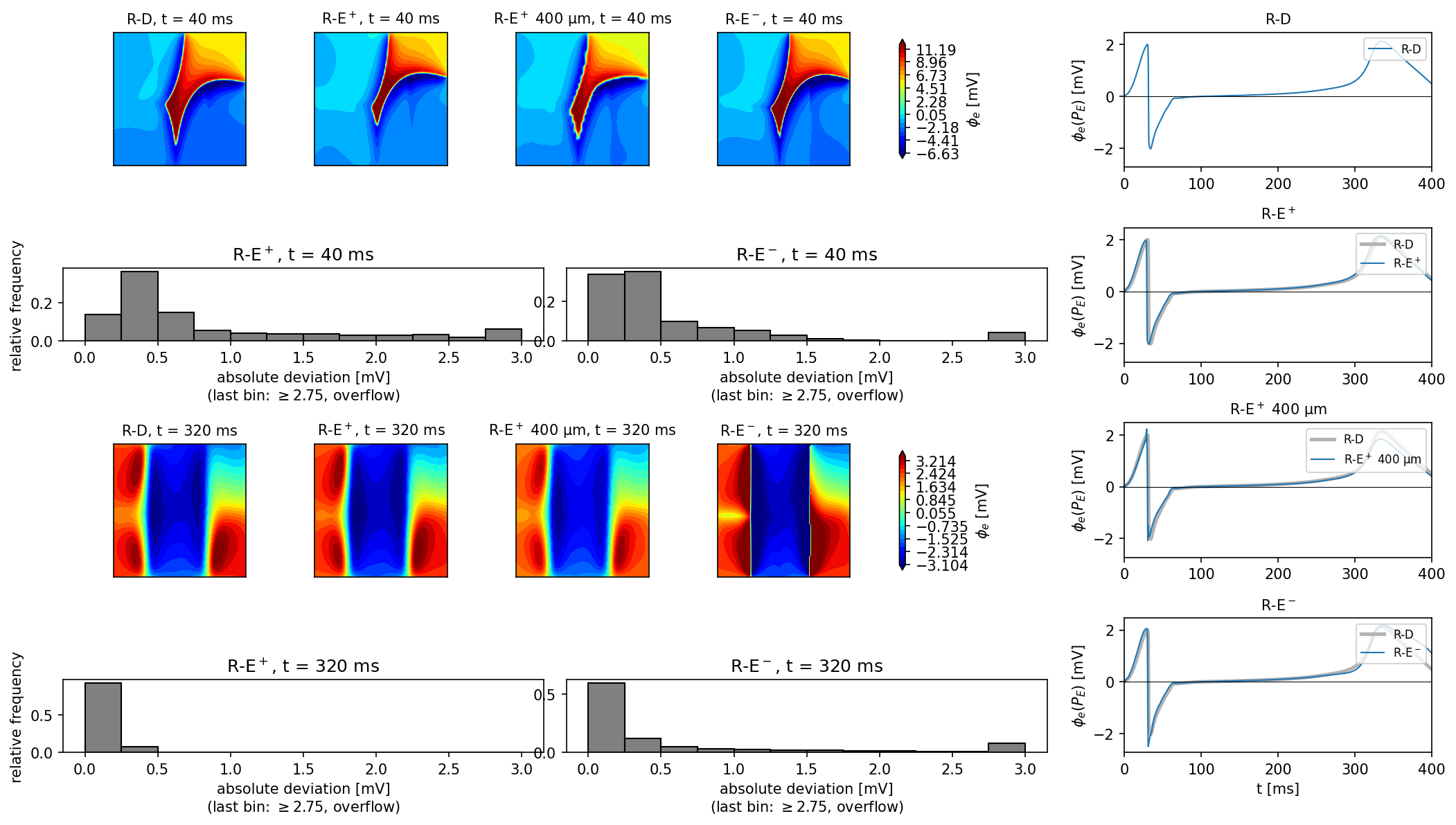
Left: \(\phi_e\) on the mid-plane at 40 and 320 ms for R-D, R-E\(^+\) (100 and 400 µm) and R-E\(^-\), with histograms of the deviation from R-D at 100 µm; right: the electrogram at \(P_E\). At 40 ms, 90% (95%) of the R-E\(^+\) potentials are within 2.4 mV (8.9 mV) of R-D and 90% (95%) of the R-E\(^-\) potentials within 1.2 mV (1.8 mV); at 320 ms the numbers are 0.22 mV (0.30 mV) for R-E\(^+\) and 2.3 mV (3.5 mV) for R-E\(^-\). The paper reports 0.25 mV and 0.75 mV for 90% of R-E\(^+\) and 95% of R-E\(^-\) at 40 ms, so both of our deviations at 40 ms are larger than the paper’s: R-E\(^+\) by about a factor 10 (2.4 against 0.25 mV) and R-E\(^-\) by about a factor 2.4 (1.8 against 0.75 mV). Our R-E\(^+\) tail at 40 ms is dominated by the thin depolarization front: the 2 ms earlier eikonal activation (see the activation demo) probably shifts the steep \(\phi_e\) front, which gives large point-wise differences in a narrow band. The median deviation is 0.50 mV, still about twice the paper’s 90% bound, so the disagreement is not confined to the tail. The electrograms of R-E\(^+\) lie on top of R-D, also at 400 µm (peak-to-peak 4.17 and 4.31 mV against 4.15 mV for R-D); R-E\(^-\) has a deeper negative peak (\(-2.50\) against \(-2.03\) mV) and a late deflection that peaks 1.5 ms later and is slightly larger than R-D (2.19 against 2.13 mV), and it stays higher until the end (1.25 against 0.61 mV at 395 ms), qualitatively as in the paper. As a check, the maps at \(P_E\) equal the electrogram samples (for example \(-1.395\) mV for R-D at 40 ms).

The amplitudes differ from the paper’s Fig. 7C, where the electrogram at \(P_E\) ranges from about \(-8\) to \(+5\) mV during depolarization and reaches about 5 mV near 300 ms; ours peaks at about \(\pm 2\) mV (R-D: \(-2.03\) and \(2.13\) mV), although our \(\phi_e\) maps cover about the same color range as the paper’s (about \(-7\) to \(15\) mV against \(-10\) to \(15\) mV). The solver chain is exact (the potential at \(P_E\) agrees to \(10^{-10}\) between three independent routes), so the difference is in the setup, which the paper only partly specifies. We measured the sensitivity with R-D at 400 µm and other electrodes: \(P_E\) at the center of the endocardial face, 1 mm bath: peak-to-peak 4.2 mV (range \(-2.3\) to \(1.9\) mV); \(P_E\) moved 0.5 mm into the bath: 3.7 mV; a point on the top face \(z = 5\) mm above the endocardial layer (\(x = 22.5\) mm): 6.1 mV (\(-2.6\) to \(3.6\) mV); points on the endocardial face closer to the S3 corner (\(y = 3\) and \(6.25\) mm): 7.0 and 6.5 mV (\(-4.5\) to \(2.6\) mV). With a 2 mm instead of 1 mm bath, \(P_E\) gives 4.0 mV and the late deflection falls from 1.9 to 1.2 mV. So the amplitude is sensitive to the electrode position (by a factor of up to 1.7 in the depolarization peaks) and to the bath size, and the unspecified placement of \(P_E\) and bath size in the paper can plausibly explain part of the difference, though not all: no electrode we tried reaches the paper’s \(-8\) mV or the 5 mV late deflection. We do not know which of these, or of other unstated details (for example the potential reference, which we take as zero mean over the bath box), accounts for the rest.