Spiral wave breakup in a 2D sheet of human ventricular tissue

In the spiral wave demo we saw that the default ten Tusscher–Panfilov 2006 (TP06) cell model gives a single, stable (although meandering) spiral wave. In this demo we reproduce one of the key results of the paper that introduced the TP06 model [tTP06]: if we change a few ionic current parameters so that the action potential duration (APD) depends more steeply on the preceding diastolic interval, the same spiral wave becomes unstable and breaks up into many smaller spirals. This is the mechanism by which a single spiral wave (ventricular tachycardia) is thought to degenerate into ventricular fibrillation.

The APD restitution curve gives the APD as a function of the preceding diastolic interval (DI), the time the tissue spends at rest between two beats. A rotating spiral constantly paces the tissue in front of it at a high rate. If the slope of the restitution curve is larger than one, a small shortening of the DI gives an even larger shortening of the next APD, which gives a longer DI, and so on. These oscillations in APD (alternans) grow until the wavefront runs into tissue that has not yet recovered, and the wave breaks [tTP06].

Note: this simulation is expensive (a \(25 \times 25\) cm sheet, simulated for 4 s), so we only simulate the first 10 ms by default, and show results from a precomputed simulation with end_time = 4000.0 at the end of the demo. That simulation was run in parallel with mpirun -n 16 python spiral_wave_breakup.py.

import shutil
from pathlib import Path

from mpi4py import MPI

import dolfinx
import gotranx
import matplotlib.pyplot as plt
import numpy as np
from matplotlib.animation import PillowWriter
from matplotlib.tri import Triangulation

import beat

comm = MPI.COMM_WORLD
results_folder = Path("results-spiral-wave-breakup")
results_folder.mkdir(exist_ok=True)

Parameters

We follow the setup in [tTP06]: a \(25 \times 25\) cm sheet of isotropic tissue, simulated for 4 s. The paper uses a grid spacing of 0.25 mm and a time step of 0.02 ms; we use a mesh size of 0.5 mm and a time step of 0.05 ms, as in the spiral wave demo. In a smaller sheet, the spiral still breaks up, but the resulting waves quickly collide with the boundaries and die out (try L = 150).

L = 250.0  # Side length of the square (mm)
h = 0.5  # Mesh size (mm)
dt = 0.05  # Time step (ms)
end_time = 10.0  # Simulation time (ms). Set to 4000.0 to reproduce the results below
t_S2 = 470.0  # Start time of the S2 stimulus (ms)

Cell model

ten Tusscher and Panfilov [tTP06] change the maximal conductances of the rapid and slow delayed rectifier potassium currents (\(G_{Kr}\), \(G_{Ks}\)), and of the plateau calcium and potassium currents (\(G_{pCa}\), \(G_{pK}\)), and scale the time constant \(\tau_f\) of the voltage dependent inactivation gate of the L-type calcium current for \(V > 0\). This gives four parameter sets, named after the maximal slope of their APD restitution curve (Table 2 in [tTP06]). Conductances are in nS/pF, except \(G_{pCa}\) which is in pA/pF, and the last column gives the behaviour of a spiral wave in 2D tissue reported in the paper:

Slope	\(G_{Kr}\)	\(G_{Ks}\)	\(G_{pCa}\)	\(G_{pK}\)	\(\tau_f\) scaling	Spiral wave
0.7	0.134	0.270	0.0619	0.0730	0.6	Stable
1.1 (default)	0.153	0.392	0.1238	0.0146	1.0	Stable (meandering)
1.4	0.172	0.441	0.3714	0.0073	1.5	Stable
1.8	0.172	0.441	0.8666	0.00219	2.0	Breakup after 2.16 s

Here we use the last parameter set.

parameter_sets = {
    "slope_0.7": dict(g_Kr=0.134, g_Ks=0.270, g_pCa=0.0619, g_pK=0.0730, tau_f_scale=0.6),
    "slope_1.1": dict(g_Kr=0.153, g_Ks=0.392, g_pCa=0.1238, g_pK=0.0146, tau_f_scale=1.0),
    "slope_1.4": dict(g_Kr=0.172, g_Ks=0.441, g_pCa=0.3714, g_pK=0.0073, tau_f_scale=1.5),
    "slope_1.8": dict(g_Kr=0.172, g_Ks=0.441, g_pCa=0.8666, g_pK=0.00219, tau_f_scale=2.0),
}
parameter_set = "slope_1.8"

The conductances are already parameters of the model, but the \(\tau_f\) scaling is not. We therefore add a parameter tau_f_scale to a copy of the .ode file, which multiplies \(\tau_f\) for \(V > 0\), before generating code for it with gotranx. With tau_f_scale = 1 the model is identical to the original one.

model_path = Path("tentusscher_panfilov_2006_epi_cell_tau_f.py")
if not model_path.is_file():
    here = Path.cwd()
    ode_text = (
        here
        / ".."
        / "odes"
        / "tentusscher_panfilov_2006"
        / "tentusscher_panfilov_2006_epi_cell.ode"
    ).read_text()
    tau_f = (
        "1102.5*exp(-((V + 27)**2)/225) + 200/(1 + exp((13 - V)/10)) "
        "+ 180/(1 + exp((V + 30)/10)) + 20"
    )
    f_gate = 'expressions("L_type Ca current", "f gate")\n'
    assert ode_text.count(f"tau_f = {tau_f} # ms") == 1
    assert ode_text.count(f_gate) == 1
    ode_text = ode_text.replace(
        f_gate,
        'parameters("L_type Ca current", "f gate",\n           tau_f_scale = 1.0)\n\n' + f_gate,
    ).replace(
        f"tau_f = {tau_f} # ms",
        f"tau_f = Conditional(Gt(V, 0), tau_f_scale, 1)*({tau_f}) # ms",
    )
    ode_path = model_path.with_suffix(".ode")
    ode_path.write_text(ode_text)
    code = gotranx.cli.gotran2py.get_code(
        gotranx.load_ode(ode_path),
        scheme=[gotranx.schemes.Scheme.generalized_rush_larsen],
    )
    model_path.write_text(code)

2026-10-20 17:33:49 [info     ] Load ode tentusscher_panfilov_2006_epi_cell_tau_f.ode

2026-10-20 17:33:49 [warning  ] Dropping a guard whose replacement failed its numeric check value=0 var=Ca_i

2026-10-20 17:33:49 [warning  ] Dropping a guard whose replacement failed its numeric check value=0 var=Na_i

2026-10-20 17:33:49 [warning  ] Dropping a guard whose replacement failed its numeric check value=0 var=K_i

2026-10-20 17:33:50 [info     ] Num states 19                 

2026-10-20 17:33:50 [info     ] Num parameters 54             

import tentusscher_panfilov_2006_epi_cell_tau_f as model

parameters = model.init_parameter_values(stim_amplitude=0.0, **parameter_sets[parameter_set])
init_states = model.init_state_values()
v_index = model.state_index("V")

Geometry, stimulus and conductivity

The rest of the setup is the same as in the spiral wave demo, so we refer to that demo for the details: a cross-field S1–S2 protocol with S1 along the left edge and S2 in the lower left quadrant, and an isotropic diffusion coefficient \(D = M / C_m\) that gives a planar conduction velocity close to the 68 cm/s in [tTP06]. The S2 stimulus is applied when the back of the S1 wave has passed the middle of the sheet, which is later than in the spiral wave demo since the sheet is larger.

N = int(round(L / h))
mesh = dolfinx.mesh.create_rectangle(
    comm,
    [[0.0, 0.0], [L, L]],
    [N, N],
    dolfinx.mesh.CellType.triangle,
)

S1_marker = 1
S2_marker = 2
tol = 1e-8


def S1_subdomain(x):
    return x[0] <= 1.0 + tol


def S2_subdomain(x):
    return np.logical_and(x[0] <= L / 2 + tol, x[1] <= L / 2 + tol)


tdim = mesh.topology.dim
S1_cells = dolfinx.mesh.locate_entities(mesh, tdim, S1_subdomain)
S2_cells = np.setdiff1d(dolfinx.mesh.locate_entities(mesh, tdim, S2_subdomain), S1_cells)
cells = np.concatenate([S1_cells, S2_cells])
values = np.concatenate(
    [np.full(len(S1_cells), S1_marker), np.full(len(S2_cells), S2_marker)],
).astype(np.int32)
order = np.argsort(cells)
stim_tags = dolfinx.mesh.meshtags(mesh, tdim, cells[order], values[order])

chi = beat.units.ureg.Quantity(1400.0, "cm**-1")
C_m = beat.units.ureg.Quantity(1.0, "uF/cm**2").to("uF/mm**2").magnitude

time = dolfinx.fem.Constant(mesh, 0.0)
I_s = [
    beat.stimulation.define_stimulus(
        mesh=mesh,
        chi=chi,
        time=time,
        subdomain_data=stim_tags,
        marker=marker,
        mesh_unit="mm",
        amplitude=50_000.0,
        start=start,
        duration=duration,
    )
    for marker, start, duration in [(S1_marker, 0.0, 2.0), (S2_marker, t_S2, 5.0)]
]

D = 0.122  # mm^2 / ms
M = D * C_m

Solvers

pde = beat.MonodomainModel(
    time=time,
    mesh=mesh,
    M=M,
    I_s=I_s,
    C_m=C_m,
    dx=I_s[0].dZ,
    params={
        "petsc_options": {
            "ksp_type": "cg",
            "pc_type": "hypre",
            "pc_hypre_type": "boomeramg",
        },
    },
)
ode = beat.odesolver.DolfinODESolver(
    v_ode=dolfinx.fem.Function(dolfinx.fem.functionspace(mesh, ("P", 1))),
    v_pde=pde.state,
    fun=model.generalized_rush_larsen,
    init_states=init_states,
    parameters=parameters,
    num_states=len(init_states),
    v_index=v_index,
)
solver = beat.MonodomainSplittingSolver(pde=pde, ode=ode)
v = solver.pde.v

Counting spiral tips

We use the same tip tracking as in the spiral wave demo: a tip is an intersection of the iso-potential line \(v = V_{iso}\) and the line \(\partial v / \partial t = 0\) [FK98]. Once the spiral breaks up, there are several tips at the same time, so the number of tips tells us when the first wave break happens. A wave that ends at the boundary of the sheet also gives an intersection there; since this is not a spiral tip, we ignore points that are closer than 5 mm to the boundary.

V_iso = -40.0  # mV
Vh = v.function_space
num_owned_cells = mesh.topology.index_map(tdim).size_local
cell_dofs = Vh.dofmap.list[:num_owned_cells]
dof_coords = Vh.tabulate_dof_coordinates()[:, :2]


def merge_points(points, radius=10.0):
    clusters: list[list[np.ndarray]] = []
    for p in points:
        for c in clusters:
            if np.linalg.norm(np.mean(c, axis=0) - p) < radius:
                c.append(p)
                break
        else:
            clusters.append([p])
    return np.array([np.mean(c, axis=0) for c in clusters]).reshape(-1, 2)


def find_tips(v_now, v_prev, boundary_distance=5.0):
    a = v_now[cell_dofs] - V_iso
    b = (v_now - v_prev)[cell_dofs]
    # Triangles where both lines pass through
    candidates = (a.min(1) < 0) & (a.max(1) > 0) & (b.min(1) < 0) & (b.max(1) > 0)
    a, b = a[candidates], b[candidates]
    x = dof_coords[cell_dofs[candidates]]
    A = np.stack(
        [
            np.stack([a[:, 1] - a[:, 0], a[:, 2] - a[:, 0]], axis=-1),
            np.stack([b[:, 1] - b[:, 0], b[:, 2] - b[:, 0]], axis=-1),
        ],
        axis=1,
    )
    rhs = -np.stack([a[:, 0], b[:, 0]], axis=-1)
    regular = np.abs(np.linalg.det(A)) > 1e-14
    xi = np.zeros_like(rhs)
    xi[regular] = np.linalg.solve(A[regular], rhs[regular][..., None])[..., 0]
    inside = regular & (xi[:, 0] >= 0) & (xi[:, 1] >= 0) & (xi.sum(axis=1) <= 1)
    points = x[:, 0] + xi[:, :1] * (x[:, 1] - x[:, 0]) + xi[:, 1:] * (x[:, 2] - x[:, 0])
    points = points[inside]
    interior = np.all((points > boundary_distance) & (points < L - boundary_distance), axis=1)
    all_points = np.vstack(comm.allgather(points[interior]))
    return merge_points(all_points)

Output

We save \(v\) to a VTX file that can be opened in ParaView. Since this demo is meant to be run in parallel, we also gather \(v\) on the first process every 20 ms and add it as a frame to an animation made with matplotlib, with the current spiral tips in red.

vtx_file = results_folder / "spiral_wave_breakup.bp"
shutil.rmtree(vtx_file, ignore_errors=True)
vtx = dolfinx.io.VTXWriter(comm, vtx_file, [v], engine="BP4")

num_owned_dofs = Vh.dofmap.index_map.size_local


def gather_v():
    """Gather the dof coordinates and values of v on rank 0."""
    data = comm.gather(np.hstack([dof_coords[:num_owned_dofs], v.x.array[:num_owned_dofs, None]]))
    return np.vstack(data) if comm.rank == 0 else None


gathered = gather_v()
if comm.rank == 0:
    triangulation = Triangulation(gathered[:, 0], gathered[:, 1])
    fig, ax = plt.subplots(figsize=(6, 6))
    image = ax.tripcolor(triangulation, gathered[:, 2], vmin=-90, vmax=40, shading="gouraud")
    (tip_markers,) = ax.plot([], [], "o", color="red", markersize=6)
    ax.set_aspect("equal")
    ax.set_axis_off()
    writer = PillowWriter(fps=15)
    writer.setup(fig, "spiral_wave_breakup.gif", dpi=60)

Time stepping

tip_every = round(1.0 / dt)
frame_every = round(20.0 / dt)

tip_time_list: list[float] = []
num_tip_list: list[int] = []
v_prev = v.x.array.copy()

t = 0.0
i = 0
num_steps = round(end_time / dt)
while i <= num_steps:
    if i % tip_every == 0:
        current_tips = find_tips(v.x.array, v_prev) if t > t_S2 + 10 else np.zeros((0, 2))
        tip_time_list.append(t)
        num_tip_list.append(len(current_tips))
        v_prev[:] = v.x.array

    if i % frame_every == 0:
        vtx.write(t)
        gathered = gather_v()
        if comm.rank == 0:
            image.set_array(gathered[:, 2])
            tip_markers.set_data(current_tips[:, 0], current_tips[:, 1])
            ax.set_title(f"t = {t:.0f} ms, {len(current_tips)} tips")
            writer.grab_frame()
            if i % (5 * frame_every) == 0:
                print(f"t = {t:.0f} ms, number of tips: {len(current_tips)}", flush=True)

    solver.step((t, t + dt))
    i += 1
    t += dt

vtx.close()
if comm.rank == 0:
    writer.finish()
    plt.close(fig)

t = 0 ms, number of tips: 0

Results

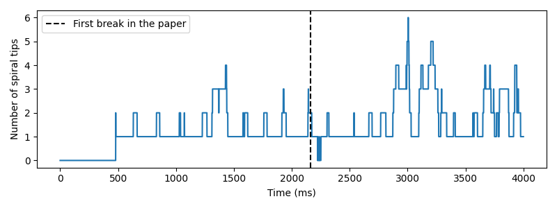
We plot the number of spiral tips over time, and report the time of the first wave break. Close to a single meandering tip, the tip detection occasionally reports two nearby points for a few milliseconds, and the S2 wavefront gives several tips while the spiral forms. We therefore define the first wave break as the first time, at least 200 ms after the S2 stimulus, that there are at least two tips for at least 50 ms in a row.

tip_times = np.array(tip_time_list)
num_tips = np.array(num_tip_list)

if comm.rank == 0:
    np.savetxt(
        results_folder / "num_tips.txt",
        np.column_stack([tip_times, num_tips]),
        header="time (ms), number of spiral tips",
    )
    fig, ax = plt.subplots(figsize=(8, 3))
    ax.plot(tip_times, num_tips)
    ax.axvline(2160.0, color="k", linestyle="--", label="First break in the paper")
    ax.set_xlabel("Time (ms)")
    ax.set_ylabel("Number of spiral tips")
    ax.legend()
    fig.tight_layout()
    fig.savefig("spiral_wave_breakup_tips.png")

    min_duration = round(50.0 / (tip_every * dt))
    several = (num_tips >= 2) & (tip_times > t_S2 + 200.0)
    # Number of consecutive samples with several tips, ending at each sample
    run_length = np.zeros(len(several), dtype=int)
    for k in range(len(several)):
        run_length[k] = several[k] * (run_length[k - 1] + 1 if k > 0 else 1)
    broken = np.flatnonzero(run_length >= min_duration)
    if len(broken) > 0:
        first_break = tip_times[broken[0] - min_duration + 1]
        print(f"First wave break at t = {first_break:.0f} ms (paper: 2160 ms)")
    else:
        print("No wave break")

No wave break

Precomputed results

Here are the results from a simulation with end_time = 4000.0.

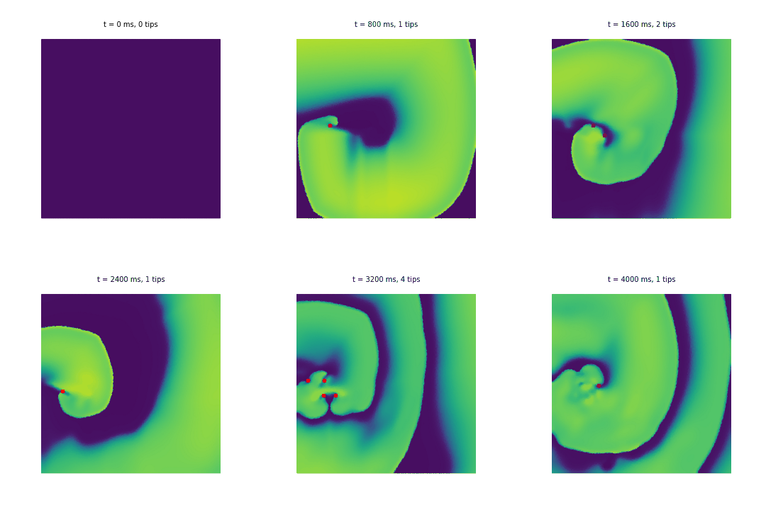
The spiral first rotates as a single spiral, similar to the one in the spiral wave demo. From about 1.3 s (the first wave break according to the definition above is at 1311 ms), the wavefront close to the spiral tip starts to break into several smaller spirals, which for a while merge back into one dominant spiral. From about 2.9 s, there are several spirals most of the time, and at the end of the simulation, waves also start to break further away from the core.

This is qualitatively the behaviour reported in [tTP06], where the first wave break for this parameter set happens at 2.16 s, after which the breakup spreads over the whole sheet. Within the 4 s we simulate, the breakup here stays more localised around the core than in the paper. Spiral breakup is known to be sensitive to the numerical resolution, and we use a coarser mesh (0.5 mm instead of 0.25 mm), a larger time step and a different numerical scheme than the paper, so the timing and extent of the breakup should not be expected to match exactly. Lowering h and dt, or simulating for longer, are good places to start if you want to explore this further.