The reaction-eikonal model: activation in a ventricular wedge

This demo reproduces the activation results (Figs. 2 and 4) of Neic et al. [NCP+17], who replace the expensive reaction-diffusion (R-D) model by a reaction-eikonal (R-E) model: an eikonal solve gives the activation time \(t_a\) (see the eikonal demo), and a foot current

\[ \frac{dv}{dt} = \frac{A}{\tau_F} e^{(t - t_a)/\tau_F}, \qquad 0 \le t - t_a \le 5\text{ ms},\; v < V_{th}, \]

with \(A = 0.91\) mV, \(\tau_F = 0.25\) ms and \(V_{th} = -30\) mV, triggers the upstroke of the cell model at \(t_a\). In R-E\(^+\) the monodomain diffusion term is kept (without stimulus); in R-E\(^-\) it is dropped, so every cell is solved on its own. The R-E models impose the prescribed conduction velocity through the eikonal solve, so, unlike R-D, they do not slow down on coarse meshes. A coarse R-D run therefore differs from the R-E runs mainly because of its own discretisation error.

The foot current is active for \(0 \le t - t_a \le 5\) ms as in openCARP; the paper’s Eq. 27 states a window before \(t_a\), which contradicts its own appendix.

Differences from the paper. Like the paper’s pseudo-bidomain models, all three models use a monodomain conductivity augmented along the surface for a 1 S/m bath (Section 8.4 of the mathematical background); the paper’s gold-standard full bidomain run is not repeated. The eikonal uses the conduction velocities measured for this R-D model at 100 µm (scripts/reaction_eikonal_cv.py) instead of the paper’s nominal 0.6/0.3 m/s. The stimulus positions are read off the paper’s figures.

To keep the documentation build short, this demo runs the three models on the 400 µm wedge for 70 ms; the results at 100/200/400 µm, computed with scripts/reaction_eikonal_wedge.py, are shown at the end.

import time as walltime
from pathlib import Path

from mpi4py import MPI

import dolfinx
import gotranx
import matplotlib.pyplot as plt
import numpy as np
import scifem

import beat
from beat.activation import ActivationTracker
from beat.eikonal import Source, solve_eikonal
from beat.reaction_eikonal import ExponentialFoot, FootCurrentODESolver

comm = MPI.COMM_WORLD
dx = 0.4  # mm
dt = 0.02  # ms
end_time = 70.0  # ms
CV_L, CV_T = 0.594, 0.324  # mm/ms, from scripts/reaction_eikonal_cv.json

Geometry, cell models and conductivities

The wedge is 25 x 25 x 5 mm with the wall across \(x\) (epicardium at \(x = 0\)), fibres rotating from -60 to +60 degrees, and 25% epicardial, 45% M and 30% endocardial cells of the ten Tusscher-Panfilov 2006 model [tTP06].

wedge = beat.geometry.get_3D_wedge_geometry(comm, dx=dx)
geo = wedge.geometry
mesh = geo.mesh
V = dolfinx.fem.functionspace(mesh, ("P", 1))
layers = beat.geometry.wedge_layer_markers(V)
g = beat.conductivities.default_conductivities("Neic2017_wedge_bath")
C_m = beat.units.ureg.Quantity(1.0, "uF/cm**2").to("uF/mm**2").magnitude
petsc_options = {"ksp_type": "cg", "pc_type": "hypre", "pc_hypre_type": "boomeramg", "ksp_rtol": 1e-8}

ode_dir = Path.cwd().parent / "odes" / "tentusscher_panfilov_2006"
cell_models = {}
for layer, name in {"EPI": "epi", "M": "M", "ENDO": "endo"}.items():
    code = gotranx.cli.gotran2py.get_code(
        gotranx.load_ode(ode_dir / f"tentusscher_panfilov_2006_{name}_cell.ode"),
        scheme=[gotranx.schemes.Scheme.generalized_rush_larsen],
    )
    namespace: dict = {}
    exec(code, namespace)
    cell_models[beat.geometry.WEDGE_LAYERS[layer]] = namespace


def cell_solver(v_pde):
    init = {k: m["init_state_values"]() for k, m in cell_models.items()}
    return beat.odesolver.DolfinMultiODESolver(
        v_ode=dolfinx.fem.Function(V),
        v_pde=v_pde,
        markers=layers,
        init_states=init,
        parameters={k: m["init_parameter_values"](stim_amplitude=0.0) for k, m in cell_models.items()},
        fun={k: m["generalized_rush_larsen"] for k, m in cell_models.items()},
        num_states={k: len(v) for k, v in init.items()},
        v_index={k: m["state_index"]("V") for k, m in cell_models.items()},
    )

2026-11-13 14:12:33 [info     ] Load ode /__w/fenicsx-beat/fenicsx-beat/odes/tentusscher_panfilov_2006/tentusscher_panfilov_2006_epi_cell.ode

2026-11-13 14:12:34 [warning  ] Dropping a guard whose replacement failed its numeric check value=0 var=Ca_i

2026-11-13 14:12:34 [warning  ] Dropping a guard whose replacement failed its numeric check value=0 var=K_i

2026-11-13 14:12:34 [warning  ] Dropping a guard whose replacement failed its numeric check value=0 var=Na_i

2026-11-13 14:12:35 [info     ] Num states 19                 

2026-11-13 14:12:35 [info     ] Num parameters 53             

2026-11-13 14:12:38 [info     ] Load ode /__w/fenicsx-beat/fenicsx-beat/odes/tentusscher_panfilov_2006/tentusscher_panfilov_2006_M_cell.ode

2026-11-13 14:12:38 [warning  ] Dropping a guard whose replacement failed its numeric check value=0 var=Ca_i

2026-11-13 14:12:38 [warning  ] Dropping a guard whose replacement failed its numeric check value=0 var=K_i

2026-11-13 14:12:38 [warning  ] Dropping a guard whose replacement failed its numeric check value=0 var=Na_i

2026-11-13 14:12:39 [info     ] Num states 19                 

2026-11-13 14:12:39 [info     ] Num parameters 53             

2026-11-13 14:12:42 [info     ] Load ode /__w/fenicsx-beat/fenicsx-beat/odes/tentusscher_panfilov_2006/tentusscher_panfilov_2006_endo_cell.ode

2026-11-13 14:12:42 [warning  ] Dropping a guard whose replacement failed its numeric check value=0 var=Ca_i

2026-11-13 14:12:42 [warning  ] Dropping a guard whose replacement failed its numeric check value=0 var=K_i

2026-11-13 14:12:42 [warning  ] Dropping a guard whose replacement failed its numeric check value=0 var=Na_i

2026-11-13 14:12:43 [info     ] Num states 19                 

2026-11-13 14:12:43 [info     ] Num parameters 53             

The activation time from the eikonal equation

The three stimuli become eikonal sources (S1 and S3 at \(t = 0\), S2 at \(t = 5\) ms).

sources = [Source((wedge.cell_tags, tag), t0) for tag, t0 in wedge.stimuli.values()]
t_a = solve_eikonal(mesh, (CV_L, CV_T, CV_T), (geo.f0, geo.s0, geo.n0), sources)

Running the three models

Each run records the activation time (instant of maximum \(dv/dt\), as in the paper) with an ActivationTracker, and \(v\) at the electrode \(P_E\) on the endocardium. beat.utils.PointEvaluator locates the probe point once, so reading \(v\) at every step is cheap.

gx, gy = np.meshgrid(np.linspace(0, 25, 101), np.linspace(0, 25, 101))
grid = np.column_stack([gx.ravel(), gy.ravel(), np.full(gx.size, 2.5)])
results: dict[str, dict] = {}
NO_ACTIVATION = 1e9  # sentinel for dofs that never activated


probe = beat.utils.PointEvaluator(mesh, wedge.electrode[None, :])


def run(name, solver, v):
    tracker = ActivationTracker(v, method="max_dvdt", t0=0.0)
    trace_t, trace = [0.0], [probe(v).item()]
    start = walltime.perf_counter()
    t = 0.0
    while t < end_time - 1e-9:
        solver.step((t, t + dt))
        t += dt
        tracker.update(t)
        trace_t.append(t)
        trace.append(probe(v).item())
    # NaN (never activated) would corrupt the MPI max reduction in evaluate_function: use a sentinel
    t_a_track = tracker.t_a  # modified in place, no ghost update needed: this is its last use
    t_a_track.x.array[np.isnan(t_a_track.x.array)] = NO_ACTIVATION
    activation = scifem.evaluate_function(t_a_track, grid).reshape(gx.shape)
    activation[~(activation < 1e3)] = np.nan  # also mixed (interpolated) cells
    results[name] = {
        "t_a": activation,
        "trace_t": np.array(trace_t),
        "trace": np.array(trace),
        "time": walltime.perf_counter() - start,
    }
    if comm.rank == 0:
        print(f"{name}: {results[name]['time']:.0f} s")
        ta = activation[np.isfinite(activation)]
        print(f"  t_a min/max {ta.min():.1f}/{ta.max():.1f}, activated {ta.size}/{activation.size}")

R-D: the monodomain model with the three stimuli. The conductivity is augmented in a layer along the surface to mimic the bath (see the electrogram demo). The layer is about 0.3 mm thick (three element rings at 100 µm, as in Bishop and Plank), so the coarser meshes use fewer rings.

time = dolfinx.fem.Constant(mesh, 0.0)
dx_layers = np.floor(0.3 / dx + 0.5 + 1e-9)
surface = beat.pseudo_bidomain.interface_layer(mesh, num_layers=max(1, int(dx_layers)))
assert geo.f0 is not None
M = beat.pseudo_bidomain.define_augmented_conductivity_tensor(f0=geo.f0, layer=surface, **g)
I_s = [
    beat.stimulation.define_stimulus(
        mesh=mesh, chi=g["chi"], time=time, subdomain_data=wedge.cell_tags, marker=tag,
        mesh_unit="mm", amplitude=50_000.0, start=t0, duration=2.0,
    )
    for tag, t0 in wedge.stimuli.values()
]
pde = beat.MonodomainModel(
    time=time, mesh=mesh, M=M, I_s=I_s, C_m=C_m, dx=I_s[0].dZ,
    params={"petsc_options": petsc_options},
)
run("R-D", beat.SplittingSolver(pde=pde, ode=cell_solver(pde.state)), pde.v)

R-D: 162 s
  t_a min/max 1.2/64.5, activated 10201/10201

R-E\(^+\): the same PDE without stimulus; the cell model is wrapped in a FootCurrentODESolver.

time = dolfinx.fem.Constant(mesh, 0.0)
pde = beat.MonodomainModel(time=time, mesh=mesh, M=M, C_m=C_m, params={"petsc_options": petsc_options})
ode = FootCurrentODESolver(cell_solver(pde.state), t_a, ExponentialFoot())
run("R-E+", beat.SplittingSolver(pde=pde, ode=ode), pde.v)

R-E+: 163 s
  t_a min/max 1.1/60.7, activated 10201/10201

R-E\(^-\): only the cell models, driven by the foot current; no linear solves at all.

solver = beat.SplittingSolver(
    pde=None,
    ode=FootCurrentODESolver(cell_solver(dolfinx.fem.Function(V)), t_a, ExponentialFoot()),
)
run("R-E-", solver, solver.v)

R-E-: 108 s
  t_a min/max 1.1/64.2, activated 10201/10201

Activation maps and deviations (400 µm)

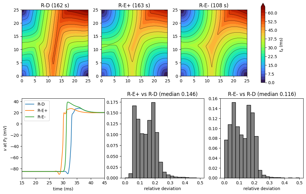
The maps show the mid-plane \(z = 2.5\) mm. The histograms show the relative deviation \(|t_{a,R-D} - t_{a,R-E}| / t_{a,R-D}\) (paper Eq. 33) of the R-E models from R-D at the same resolution (away from the sources, where it is undefined). At 400 µm, R-D is the slower model: its activation is delayed by the coarse mesh, while R-E keeps the 100 µm conduction velocities. These histograms therefore measure mostly the discretisation error of R-D, not that of R-E; the meaningful accuracy comparison is against R-D at 100 µm, shown in the precomputed figure below (as in the paper’s Fig. 2).

if comm.rank == 0:
    fig, axes = plt.subplots(2, 3, figsize=(12, 7.5))
    for ax, name in zip(axes[0], results):
        c = ax.contourf(gx, gy, results[name]["t_a"], levels=np.linspace(0, 65, 27), cmap="turbo", extend="max")
        ax.contour(gx, gy, results[name]["t_a"], levels=np.arange(0, 70, 5), colors="k", linewidths=0.4)
        ax.set_title(f"{name} ({results[name]['time']:.0f} s)")
        ax.set_aspect("equal")
    fig.colorbar(c, ax=axes[0], label="$t_a$ (ms)")
    ref = results["R-D"]["t_a"]
    mask = ref > 1.0
    for ax, name in zip(axes[1, 1:], ("R-E+", "R-E-")):
        drel = np.abs(ref - results[name]["t_a"])[mask] / ref[mask]
        drel = drel[np.isfinite(drel)]
        ax.hist(
            drel, bins=np.linspace(0, 0.5, 21), weights=np.full(drel.size, 1 / drel.size),
            color="0.5", edgecolor="k",
        )
        ax.set_title(f"{name} vs R-D (median {np.median(drel):.3f})")
        print(f"{name}: median relative deviation from R-D {np.median(drel):.3f}, max {drel.max():.3f}")
        ax.set_xlabel("relative deviation")
    ax = axes[1, 0]
    for name in results:
        ax.plot(results[name]["trace_t"], results[name]["trace"], label=name)
    ax.set_xlim(15, 45)
    ax.set_xlabel("time (ms)")
    ax.set_ylabel("$v$ at $P_E$ (mV)")
    ax.legend()
    fig.savefig("reaction_eikonal_wedge_activation.png")

R-E+: median relative deviation from R-D 0.146, max 0.463
R-E-: median relative deviation from R-D 0.116, max 0.487

Precomputed results at 100, 200 and 400 µm

The figures below come from scripts/reaction_eikonal_wedge.py (run with MPI at each resolution) and scripts/reaction_eikonal_wedge_figures.py. As in the paper’s Fig. 2, the R-D activation slows down on coarser meshes, while R-E\(^+\) and R-E\(^-\) keep the prescribed conduction velocity; the histograms compare the 400 µm runs with R-D at 100 µm.

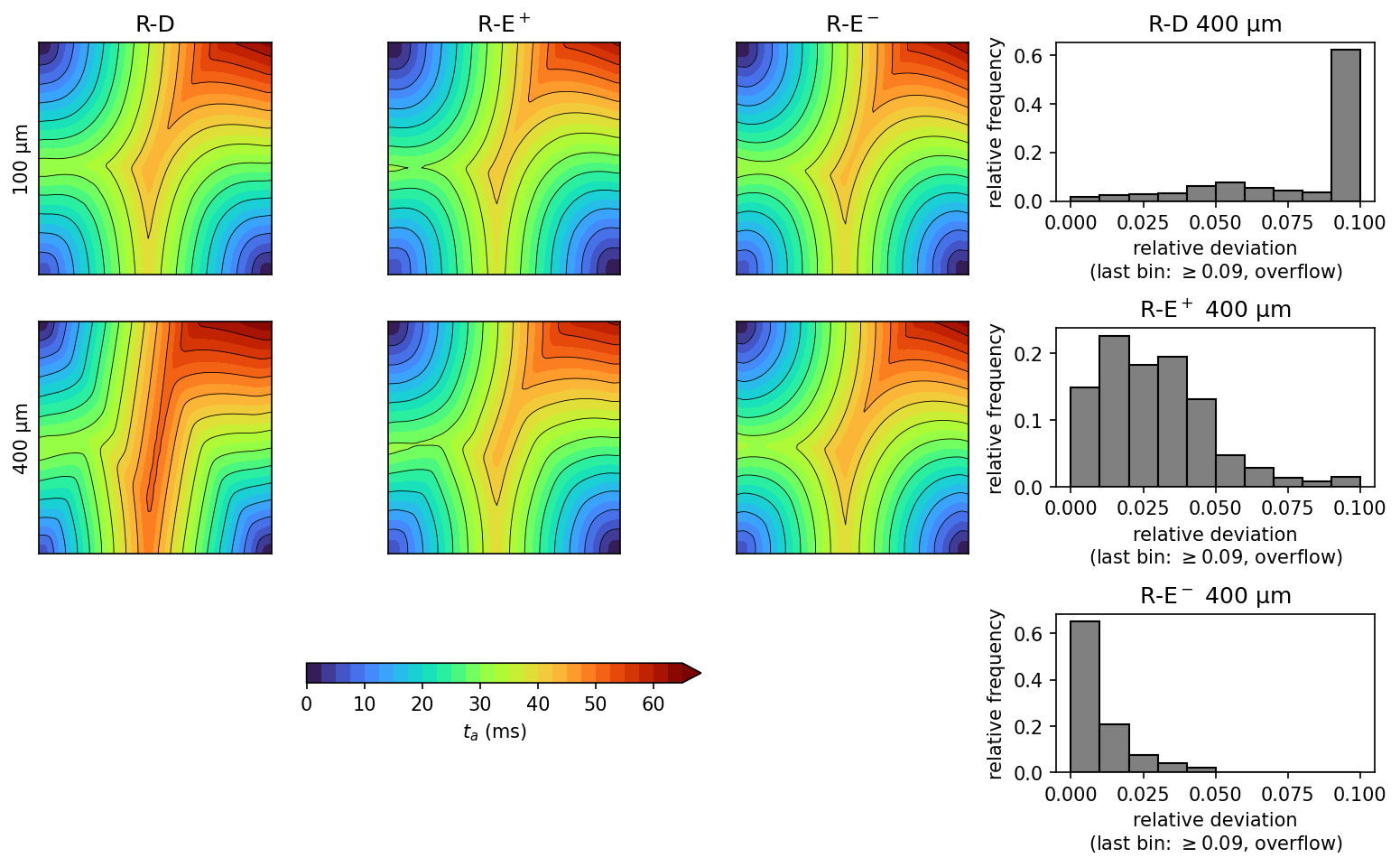
Against R-D at 100 µm, the median relative deviation of the activation time is 13% (90% of the points below 25%) for R-D at 400 µm, 2.7% (90% below 5.2%) for R-E\(^+\) at 400 µm and 0.8% (90% below 2.5%) for R-E\(^-\) at 400 µm; at 200 µm it is 1.5% for R-D. R-E\(^+\) at 200 µm has a median of 7.4%, larger than at 400 µm, because its activation is systematically early: with the bath layer the 100 µm R-D wave is slower than the eikonal wave at the measured velocities, which are unchanged. The size of the augmentation layer matters little: with three rings at every resolution (instead of a constant 0.3 mm) the 400 µm R-D median would be 10.9% and R-E\(^+\) 3.0%. In the 100 µm panels R-E\(^+\) shows a small kink in the contours at the left edge.

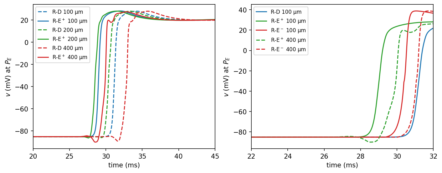
The upstrokes at \(P_E\) (cf. the paper’s Fig. 4): R-D at 200 and 400 µm activates late, the R-E models do not; R-E\(^-\) has a faster upstroke and a larger overshoot because it ignores diffusion. The upstroke at \(P_E\) occurs at 31.3 ms (R-D), 29.1 ms (R-E\(^+\)) and 30.5 ms (R-E\(^-\)) at 100 µm, and at 33.0, 30.0 and 31.2 ms at 400 µm: the R-E times hardly depend on the mesh, whereas R-D is delayed by 1.7 ms. The R-E\(^+\) and R-E\(^-\) times differ from R-D by about 2 ms and 0.8 ms (100 µm).